C51

Overview

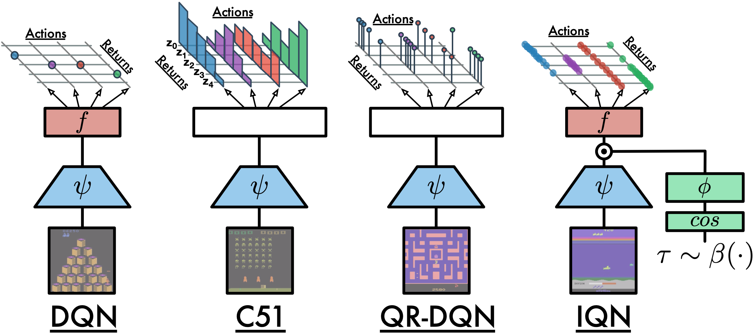
C51 was first proposed in A Distributional Perspective on Reinforcement Learning, different from previous works, C51 evaluates the complete distribution of a q-value rather than only the expectation. The authors designed a distributional Bellman operator, which preserves multimodality in value distributions and is believed to achieve more stable learning and mitigates the negative effects of learning from a non-stationary policy.

Quick Facts

1. C51 is a model-free and value-based RL algorithm.

2. C51 only support discrete action spaces.

3. C51 is an off-policy algorithm.

4. Usually, C51 use eps-greedy or multinomial sample for exploration.

5. C51 can be equipped with RNN.

Pseudo-code

Note

C51 models the value distribution using a discrete distribution, whose support set are N atoms: \(z_i = V_min + i * delta, i = 0,1,...,N-1\) and \(delta = (V_\max - V_\min) / N\). Each atom \(z_i\) has a parameterized probability \(p_i\). The Bellman update of C51 projects the distribution of \(r + \gamma * z_j^(t+1)\) onto the distribution \(z_i^t\).

Key Equations or Key Graphs

The Bellman target of C51 is derived by projecting the returned distribution \(r + \gamma * z_j\) onto the current distribution \(z_i\). Given a sample transition \((x, a, r, x')\), we compute the Bellman update \(Tˆz_j := r + \gamma z_j\) for each atom \(z_j\), then distribute its probability \(p_{j}(x', \pi(x'))\) to the immediate neighbors \(p_{i}(x, \pi(x))\):

\[\left(\Phi \hat{T} Z_{\theta}(x, a)\right)_{i}=\sum_{j=0}^{N-1}\left[1-\frac{\left|\left[\hat{\mathcal{T}} z_{j}\right]_{V_{\mathrm{MIN}}}^{V_{\mathrm{MAX}}}-z_{i}\right|}{\Delta z}\right]_{0}^{1} p_{j}\left(x^{\prime}, \pi\left(x^{\prime}\right)\right)\]

Extensions

• C51s can be combined with:

  • PER (Prioritized Experience Replay)

  • Multi-step TD-loss

  • Double (target) network

  • Dueling head

  • RNN

Implementation

Tip

Our benchmark result of C51 uses the same hyper-parameters as DQN except the exclusive n_atom of C51, which is empirically set as 51.

The default config of C51 is defined as follows:

class ding.policy.c51.C51Policy(cfg: dict, model: Optional[Union[type, torch.nn.modules.module.Module]] = None, enable_field: Optional[List[str]] = None)

Overview:

Policy class of C51 algorithm.

Config:

ID	Symbol	Type	Default Value	Description	Other(Shape)
1	type	str	c51	RL policy register name, refer to registry POLICY_REGISTRY	this arg is optional, a placeholder
2	cuda	bool	False	Whether to use cuda for network	this arg can be diff- erent from modes
3	on_policy	bool	False	Whether the RL algorithm is on-policy or off-policy
4	priority	bool	False	Whether use priority(PER)	priority sample, update priority
5	model.v_min	float	-10	Value of the smallest atom in the support set.
6	model.v_max	float	10	Value of the largest atom in the support set.
7	model.n_atom	int	51	Number of atoms in the support set of the value distribution.
8	other.eps .start	float	0.95	Start value for epsilon decay.
9	other.eps .end	float	0.1	End value for epsilon decay.
10	discount_ factor	float	0.97, [0.95, 0.999]	Reward’s future discount factor, aka. gamma	may be 1 when sparse reward env
11	nstep	int	1,	N-step reward discount sum for target q_value estimation
12	learn.update per_collect	int	3	How many updates(iterations) to train after collector’s one collection. Only valid in serial training	this args can be vary from envs. Bigger val means more off-policy

The network interface C51 used is defined as follows:

class ding.model.template.q_learning.C51DQN(obs_shape: Union[int, ding.utils.type_helper.SequenceType], action_shape: Union[int, ding.utils.type_helper.SequenceType], encoder_hidden_size_list: ding.utils.type_helper.SequenceType = [128, 128, 64], head_hidden_size: Optional[int] = None, head_layer_num: int = 1, activation: Optional[torch.nn.modules.module.Module] = ReLU(), norm_type: Optional[str] = None, v_min: Optional[float] = - 10, v_max: Optional[float] = 10, n_atom: Optional[int] = 51)

__init__(obs_shape: Union[int, ding.utils.type_helper.SequenceType], action_shape: Union[int, ding.utils.type_helper.SequenceType], encoder_hidden_size_list: ding.utils.type_helper.SequenceType = [128, 128, 64], head_hidden_size: Optional[int] = None, head_layer_num: int = 1, activation: Optional[torch.nn.modules.module.Module] = ReLU(), norm_type: Optional[str] = None, v_min: Optional[float] = - 10, v_max: Optional[float] = 10, n_atom: Optional[int] = 51) → None

Overview:

Init the C51 Model according to input arguments.

Arguments:

• obs_shape (Union[int, SequenceType]): Observation’s space.

• action_shape (Union[int, SequenceType]): Action’s space.

• encoder_hidden_size_list (SequenceType): Collection of hidden_size to pass to Encoder

• head_hidden_size (Optional[int]): The hidden_size to pass to Head.

• head_layer_num (int): The num of layers used in the network to compute Q value output

• activation (Optional[nn.Module]):

  The type of activation function to use in MLP the after layer_fn, if None then default set to nn.ReLU()

• norm_type (Optional[str]):

  The type of normalization to use, see ding.torch_utils.fc_block for more details`

• n_atom (Optional[int]): Number of atoms in the prediction distribution.

forward(x: torch.Tensor) → Dict

Overview:

Use observation tensor to predict C51DQN’s output. Parameter updates with C51DQN’s MLPs forward setup.

Arguments:

• x (torch.Tensor):

  The encoded embedding tensor w/ (B, N=head_hidden_size).

Returns:

• outputs (Dict):

  Run with encoder and head. Return the result prediction dictionary.

ReturnsKeys:

• logit (torch.Tensor): Logit tensor with same size as input x.

• distribution (torch.Tensor): Distribution tensor of size (B, N, n_atom)

Shapes:

• x (torch.Tensor): \((B, N)\), where B is batch size and N is head_hidden_size.

• logit (torch.FloatTensor): \((B, M)\), where M is action_shape.

• distribution(torch.FloatTensor): \((B, M, P)\), where P is n_atom.

Examples:

>>> model = C51DQN(128, 64)  # arguments: 'obs_shape' and 'action_shape'
>>> inputs = torch.randn(4, 128)
>>> outputs = model(inputs)
>>> assert isinstance(outputs, dict)
>>> # default head_hidden_size: int = 64,
>>> assert outputs['logit'].shape == torch.Size([4, 64])
>>> # default n_atom: int = 51
>>> assert outputs['distribution'].shape == torch.Size([4, 64, 51])

The bellman updates of C51 is implemented as:

The Benchmark result of C51 implemented in DI-engine is shown in Benchmark

QRDQN

Overview

QR(Quantile Regression)DQN was proposed in Distributional Reinforcement Learning with Quantile Regression and inherits the idea of learning the distribution of a q-value. Instead of approximate the distribution density function with discrete atoms, QRDQN, direct regresses a discrete set of quantiles of a q-value.

Quick Facts

1. QRDQN is a model-free and value-based RL algorithm.

2. QRDQN only support discrete action spaces.

3. QRDQN is an off-policy algorithm.

4. Usually, QRDQN use eps-greedy or multinomial sample for exploration.

5. QRDQN can be equipped with RNN.

Key Equations or Key Graphs

The quantile regression loss, for a quantile tau in \([0, 1]\), is an asymmetric convex loss function that penalizes overestimation errors with weight \(\tau\) and underestimation errors with weight \(1−\tau\). For a distribution Z, and a given quantile tau, the value of the quantile function \(F_Z^−1(\tau)\) may be characterized as the minimizer of the quantile regression loss:

\[\begin{split}\begin{array}{r} \mathcal{L}_{\mathrm{QR}}^{\tau}(\theta):=\mathbb{E}_{\hat{z} \sim Z}\left[\rho_{\tau}(\hat{Z}-\theta)\right], \text { where } \\ \rho_{\tau}(u)=u\left(\tau-\delta_{\{u<0\}}\right), \forall u \in \mathbb{R} \end{array}\end{split}\]

Pseudo-code

Note

The quantile huber loss is applied during the Bellman update of QRDQN.

Extensions

QRDQN can be combined with:

• PER (Prioritized Experience Replay)

• Multi-step TD-loss

• Double (target) network

• RNN

Implementation

Tip

Our benchmark result of QRDQN uses the same hyper-parameters as DQN except the QRDQN’s exclusive hyper-parameter, the number of quantiles, which is empirically set as 32.

The default config of QRDQN is defined as follows:

class ding.policy.qrdqn.QRDQNPolicy(cfg: dict, model: Optional[Union[type, torch.nn.modules.module.Module]] = None, enable_field: Optional[List[str]] = None)

Overview:

Policy class of QRDQN algorithm.

Config:

ID	Symbol	Type	Default Value	Description	Other(Shape)
1	type	str	qrdqn	RL policy register name, refer to registry POLICY_REGISTRY	this arg is optional, a placeholder
2	cuda	bool	False	Whether to use cuda for network	this arg can be diff- erent from modes
3	on_policy	bool	False	Whether the RL algorithm is on-policy or off-policy
4	priority	bool	True	Whether use priority(PER)	priority sample, update priority
6	other.eps .start	float	0.05	Start value for epsilon decay. It’s small because rainbow use noisy net.
7	other.eps .end	float	0.05	End value for epsilon decay.
8	discount_ factor	float	0.97, [0.95, 0.999]	Reward’s future discount factor, aka. gamma	may be 1 when sparse reward env
9	nstep	int	3, [3, 5]	N-step reward discount sum for target q_value estimation
10	learn.update per_collect	int	3	How many updates(iterations) to train after collector’s one collection. Only valid in serial training	this args can be vary from envs. Bigger val means more off-policy
11	learn.kappa	float	/	Threshold of Huber loss

The network interface QRDQN used is defined as follows:

class ding.model.template.q_learning.QRDQN(obs_shape: Union[int, ding.utils.type_helper.SequenceType], action_shape: Union[int, ding.utils.type_helper.SequenceType], encoder_hidden_size_list: ding.utils.type_helper.SequenceType = [128, 128, 64], head_hidden_size: Optional[int] = None, head_layer_num: int = 1, num_quantiles: int = 32, activation: Optional[torch.nn.modules.module.Module] = ReLU(), norm_type: Optional[str] = None)

__init__(obs_shape: Union[int, ding.utils.type_helper.SequenceType], action_shape: Union[int, ding.utils.type_helper.SequenceType], encoder_hidden_size_list: ding.utils.type_helper.SequenceType = [128, 128, 64], head_hidden_size: Optional[int] = None, head_layer_num: int = 1, num_quantiles: int = 32, activation: Optional[torch.nn.modules.module.Module] = ReLU(), norm_type: Optional[str] = None) → None

Overview:

Init the QRDQN Model according to input arguments.

Arguments:

• obs_shape (Union[int, SequenceType]): Observation’s space.

• action_shape (Union[int, SequenceType]): Action’s space.

• encoder_hidden_size_list (SequenceType): Collection of hidden_size to pass to Encoder

• head_hidden_size (Optional[int]): The hidden_size to pass to Head.

• head_layer_num (int): The num of layers used in the network to compute Q value output

• num_quantiles (int): Number of quantiles in the prediction distribution.

• activation (Optional[nn.Module]):

  The type of activation function to use in MLP the after layer_fn, if None then default set to nn.ReLU()

• norm_type (Optional[str]):

  The type of normalization to use, see ding.torch_utils.fc_block for more details`

forward(x: torch.Tensor) → Dict

Overview:

Use observation tensor to predict QRDQN’s output. Parameter updates with QRDQN’s MLPs forward setup.

Arguments:

• x (torch.Tensor):

  The encoded embedding tensor with (B, N=hidden_size).

Returns:

• outputs (Dict):

  Run with encoder and head. Return the result prediction dictionary.

ReturnsKeys:

• logit (torch.Tensor): Logit tensor with same size as input x.

• q (torch.Tensor): Q valye tensor tensor of size (B, N, num_quantiles)

• tau (torch.Tensor): tau tensor of size (B, N, 1)

Shapes:

• x (torch.Tensor): \((B, N)\), where B is batch size and N is head_hidden_size.

• logit (torch.FloatTensor): \((B, M)\), where M is action_shape.

• tau (torch.Tensor): \((B, M, 1)\)

Examples:

>>> model = QRDQN(64, 64)
>>> inputs = torch.randn(4, 64)
>>> outputs = model(inputs)
>>> assert isinstance(outputs, dict)
>>> assert outputs['logit'].shape == torch.Size([4, 64])
>>> # default num_quantiles : int = 32
>>> assert outputs['q'].shape == torch.Size([4, 64, 32])
>>> assert outputs['tau'].shape == torch.Size([4, 32, 1])

The bellman updates of QRDQN is implemented in the function qrdqn_nstep_td_error of ding/rl_utils/td.py.

The Benchmark result of QRDQN implemented in DI-engine is shown in Benchmark

IQN

Overview

IQN was proposed in Implicit Quantile Networks for Distributional Reinforcement Learning. The key difference between IQN and QRDQN is that IQN introduces the implicit quantile network (IQN), a deterministic parametric function trained to re-parameterize samples from a base distribution, e.g. tau in U([0, 1]), to the respective quantile values of a target distribution, while QRDQN direct learns a fixed set of pre-defined quantiles.

Quick Facts

1. IQN is a model-free and value-based RL algorithm.

2. IQN only support discrete action spaces.

3. IQN is an off-policy algorithm.

4. Usually, IQN use eps-greedy or multinomial sample for exploration.

5. IQN can be equipped with RNN.

Key Equations

In implicit quantile networks, a sampled quantile tau is first encoded into an embedding vector via:

\[\phi_{j}(\tau):=\operatorname{ReLU}\left(\sum_{i=0}^{n-1} \cos (\pi i \tau) w_{i j}+b_{j}\right)\]

Then the quantile embedding is element-wise multiplied by the embedding of the observation of the environment, and the subsequent fully-connected layers map the resulted product vector to the respective quantile value.

Key Graphs

The comparison among DQN, C51, QRDQN and IQN is shown as follows:

Extensions

IQN can be combined with:

• PER (Prioritized Experience Replay)

  Tip

  Whether PER improves IQN depends on the task and the training strategy.

• Multi-step TD-loss

• Double (target) Network

• RNN

Implementation

Tip

Our benchmark result of IQN uses the same hyper-parameters as DQN except the IQN’s exclusive hyper-parameter, the number of quantiles, which is empirically set as 32. The number of quantiles are not recommended to set larger than 64, which brings marginal gain and much more forward latency.

The default config of IQN is defined as follows:

class ding.policy.iqn.IQNPolicy(cfg: dict, model: Optional[Union[type, torch.nn.modules.module.Module]] = None, enable_field: Optional[List[str]] = None)

Overview:

Policy class of IQN algorithm.

Config:

ID	Symbol	Type	Default Value	Description	Other(Shape)
1	type	str	qrdqn	RL policy register name, refer to registry POLICY_REGISTRY	this arg is optional, a placeholder
2	cuda	bool	False	Whether to use cuda for network	this arg can be diff- erent from modes
3	on_policy	bool	False	Whether the RL algorithm is on-policy or off-policy
4	priority	bool	True	Whether use priority(PER)	priority sample, update priority
6	other.eps .start	float	0.05	Start value for epsilon decay. It’s small because rainbow use noisy net.
7	other.eps .end	float	0.05	End value for epsilon decay.
8	discount_ factor	float	0.97, [0.95, 0.999]	Reward’s future discount factor, aka. gamma	may be 1 when sparse reward env
9	nstep	int	3, [3, 5]	N-step reward discount sum for target q_value estimation
10	learn.update per_collect	int	3	How many updates(iterations) to train after collector’s one collection. Only valid in serial training	this args can be vary from envs. Bigger val means more off-policy
11	learn.kappa	float	/	Threshold of Huber loss

The network interface IQN used is defined as follows:

class ding.model.template.q_learning.IQN(obs_shape: Union[int, ding.utils.type_helper.SequenceType], action_shape: Union[int, ding.utils.type_helper.SequenceType], encoder_hidden_size_list: ding.utils.type_helper.SequenceType = [128, 128, 64], head_hidden_size: Optional[int] = None, head_layer_num: int = 1, num_quantiles: int = 32, quantile_embedding_size: int = 128, activation: Optional[torch.nn.modules.module.Module] = ReLU(), norm_type: Optional[str] = None)

__init__(obs_shape: Union[int, ding.utils.type_helper.SequenceType], action_shape: Union[int, ding.utils.type_helper.SequenceType], encoder_hidden_size_list: ding.utils.type_helper.SequenceType = [128, 128, 64], head_hidden_size: Optional[int] = None, head_layer_num: int = 1, num_quantiles: int = 32, quantile_embedding_size: int = 128, activation: Optional[torch.nn.modules.module.Module] = ReLU(), norm_type: Optional[str] = None) → None

Overview:

Init the IQN Model according to input arguments.

Arguments:

• obs_shape (Union[int, SequenceType]): Observation space shape.

• action_shape (Union[int, SequenceType]): Action space shape.

• encoder_hidden_size_list (SequenceType): Collection of hidden_size to pass to Encoder

• head_hidden_size (Optional[int]): The hidden_size to pass to Head.

• head_layer_num (int): The num of layers used in the network to compute Q value output

• num_quantiles (int): Number of quantiles in the prediction distribution.

• activation (Optional[nn.Module]):

  The type of activation function to use in MLP the after layer_fn, if None then default set to nn.ReLU()

• norm_type (Optional[str]):

  The type of normalization to use, see ding.torch_utils.fc_block for more details.

forward(x: torch.Tensor) → Dict

Overview:

Use encoded embedding tensor to predict IQN’s output. Parameter updates with IQN’s MLPs forward setup.

Arguments:

• x (torch.Tensor):

  The encoded embedding tensor with (B, N=hidden_size).

Returns:

• outputs (Dict):

  Run with encoder and head. Return the result prediction dictionary.

ReturnsKeys:

• logit (torch.Tensor): Logit tensor with same size as input x.

• q (torch.Tensor): Q valye tensor tensor of size (num_quantiles, N, B)

• quantiles (torch.Tensor): quantiles tensor of size (quantile_embedding_size, 1)

Shapes:

• x (torch.Tensor): \((B, N)\), where B is batch size and N is head_hidden_size.

• logit (torch.FloatTensor): \((B, M)\), where M is action_shape

• quantiles (torch.Tensor): \((P, 1)\), where P is quantile_embedding_size.

Examples:

>>> model = IQN(64, 64) # arguments: 'obs_shape' and 'action_shape'
>>> inputs = torch.randn(4, 64)
>>> outputs = model(inputs)
>>> assert isinstance(outputs, dict)
>>> assert outputs['logit'].shape == torch.Size([4, 64])
>>> # default num_quantiles: int = 32
>>> assert outputs['q'].shape == torch.Size([32, 4, 64]
>>> # default quantile_embedding_size: int = 128
>>> assert outputs['quantiles'].shape == torch.Size([128, 1])

The bellman updates of IQN used is defined in the function iqn_nstep_td_error of ding/rl_utils/td.py.

The Benchmark result of IQN implemented in DI-engine is shown in Benchmark

References

(C51) Marc G. Bellemare, Will Dabney, Rémi Munos: “A Distributional Perspective on Reinforcement Learning”, 2017; arXiv:1707.06887. https://arxiv.org/abs/1707.06887

(QRDQN) Will Dabney, Mark Rowland, Marc G. Bellemare, Rémi Munos: “Distributional Reinforcement Learning with Quantile Regression”, 2017; arXiv:1710.10044. https://arxiv.org/pdf/1710.10044

(IQN) Will Dabney, Georg Ostrovski, David Silver, Rémi Munos: “Implicit Quantile Networks for Distributional Reinforcement Learning”, 2018; arXiv:1806.06923. https://arxiv.org/pdf/1806.06923