# YOLO V3 Objective Detection

---
## Table of Contents

- [Installation](#installation)
- [Introduction](#introduction)
- [Data preparation](#data-preparation)
- [Training](#training)
- [Evaluation](#evaluation)
- [Inference and Visualization](#inference-and-visualization)

## Installation

Running sample code in this directory requires PaddelPaddle Fluid v.1.4 and later. If the PaddlePaddle on your device is lower than this version, please follow the instructions in [installation document](http://www.paddlepaddle.org/documentation/docs/en/1.4/beginners_guide/install/index_en.html) and make an update.

## Introduction

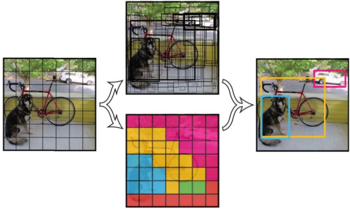
[YOLOv3](https://arxiv.org/abs/1804.02767) is a one stage end to end detector。the detection principle of YOLOv3 is as follow:
<p align="center">
<img src="image/YOLOv3.jpg" height=400 width=600 hspace='10'/> <br />
YOLOv3 detection principle
</p>

YOLOv3 divides the input image in to S\*S grids and predict B bounding boxes in each grid, predictions of boxes include Location(x, y, w, h), Confidence Score and probabilities of C classes, therefore YOLOv3 output layer has S\*S\*B\*(5 + C) channels. YOLOv3 loss consists of three parts: location loss, confidence loss and classification loss.
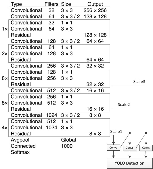
The bone network of YOLOv3 is darknet53, the structure of YOLOv3 is as follow:
<p align="center">
<img src="image/YOLOv3_structure.jpg" height=400 width=400 hspace='10'/> <br />
YOLOv3 structure
</p>

YOLOv3 networks are composed of base feature extraction network, multi-scale feature fusion layers, and output layers.

1. Feature extraction network: YOLOv3 uses [DarkNet53](https://arxiv.org/abs/1612.08242) for feature extracion. Darknet53 uses a full convolution structure, replacing the pooling layer with a convolution operation of step size 2, and adding Residual-block to avoid gradient dispersion when the number of network layers is too deep.

2. Feature fusion layer. In order to solve the problem that the previous YOLO version is not sensitive to small objects, YOLOv3 uses three different scale feature maps for target detection, which are 13\*13, 26\*26, 52\*52, respectively, for detecting large, medium and small objects. The feature fusion layer selects the three scale feature maps produced by DarkNet as input, and draws on the idea of FPN (feature pyramid networks) to fuse the feature maps of each scale through a series of convolutional layers and upsampling.

3. Output layer: The output layer also uses a full convolution structure. The number of convolution kernels in the last convolutional layer is 255:3\*(80+4+1)=255, and 3 indicates that a grid cell contains 3 bounding boxes. 4 represents the four coordinate information of the box, 1 represents the Confidence Score, and 80 represents the probability of 80 categories in the COCO dataset.

## Data preparation

Train the model on [MS-COCO dataset](http://cocodataset.org/#download), download dataset as below:

    cd dataset/coco
    ./download.sh

The data catalog structure is as follows:

```
  dataset/coco/
  ├── annotations
  │   ├── instances_train2014.json
  │   ├── instances_train2017.json
  │   ├── instances_val2014.json
  │   ├── instances_val2017.json
  |   ...
  ├── train2017
  │   ├── 000000000009.jpg
  │   ├── 000000580008.jpg
  |   ...
  ├── val2017
  │   ├── 000000000139.jpg
  │   ├── 000000000285.jpg
  |   ...
  
```

## Training

**Install the [cocoapi](https://github.com/cocodataset/cocoapi):**

To train the model, [cocoapi](https://github.com/cocodataset/cocoapi) is needed. Install the cocoapi:

    git clone https://github.com/cocodataset/cocoapi.git
    cd cocoapi/PythonAPI
    # if cython is not installed
    pip install Cython
    # Install into global site-packages
    make install
    # Alternatively, if you do not have permissions or prefer
    # not to install the COCO API into global site-packages
    python2 setup.py install --user

**download the pre-trained model:** This sample provides Resnet-50 pre-trained model which is converted from Caffe. The model fuses the parameters in batch normalization layer. One can download pre-trained model as:

    sh ./weights/download.sh

Set `pretrain` to load pre-trained model. In addition, this parameter is used to load trained model when finetuning as well.
Please make sure that pre-trained model is downloaded and loaded correctly, otherwise, the loss may be NAN during training.


**training:** After data preparation, one can start the training step by:

    python train.py \
       --model_save_dir=output/ \
       --pretrain=${path_to_pretrain_model}
       --data_dir=${path_to_data}

- Set ```export CUDA_VISIBLE_DEVICES=0,1,2,3,4,5,6,7``` to specifiy 8 GPU to train.
- For more help on arguments:

    python train.py --help

**data reader introduction:**

* Data reader is defined in `reader.py` .

**model configuration:**

* The model uses 9 anchors generated based on the COCO dataset, which are 10x13, 16x30, 33x23, 30x61, 62x45, 59x119, 116x90, 156x198, 373x326.

* NMS threshold=0.45, NMS valid=0.005 nms_topk=400, nms_posk=100

**training strategy:**

*  Use momentum optimizer with momentum=0.9.
*  In first 4000 iteration, the learning rate increases linearly from 0.0 to 0.001. Then lr is decayed at 400000, 450000 iteration with multiplier 0.1, 0.01. The maximum iteration is 500000.

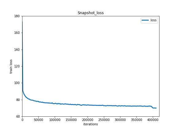
Training result is shown as below：
<p align="center">
<img src="image/train_loss.png" height="500" width="650" hspace="10"/><br />
Train Loss
</p>

## Evaluation

Evaluation is to evaluate the performance of a trained model. This sample provides `eval.py` which uses a COCO-specific mAP metric defined by [COCO committee](http://cocodataset.org/#detections-eval).

`eval.py` is the main executor for evalution, one can start evalution step by:

    python eval.py \
        --dataset=coco2017 \
        --weights=${path_to_weights} \

- Set ```export CUDA_VISIBLE_DEVICES=0``` to specifiy one GPU to eval.

Evalutaion result is shown as below:

|   input size  | mAP(IoU=0.50:0.95) | mAP(IoU=0.50) | mAP(IoU=0.75) |
| :------: | :------: | :------: | :------: |
| 608x608| 37.7 | 59.8 | 40.8 |
| 416x416 | 36.5 | 58.2 | 39.1 |
| 320x320 | 34.1 | 55.4 | 36.3 |

- **NOTE:** evaluations based on `pycocotools` evaluator, predict bounding boxes with `score < 0.05` were not filtered out. Some frameworks which filtered out predict bounding boxes with `score < 0.05` will cause a drop in accuracy.

## Inference and Visualization

Inference is used to get prediction score or image features based on trained models. `infer.py`  is the main executor for inference, one can start infer step by:

    python infer.py \
       --dataset=coco2017 \
        --weights=${path_to_weights}  \
        --image_path=data/COCO17/val2017/  \
        --image_name=000000000139.jpg \
        --draw_threshold=0.5

Inference speed:


|   input size  | 608x608 | 416x416 | 320x320 |
|:-------------:| :-----: | :-----: | :-----: |
| infer speed | 48 ms/frame | 29 ms/frame |24 ms/frame | 


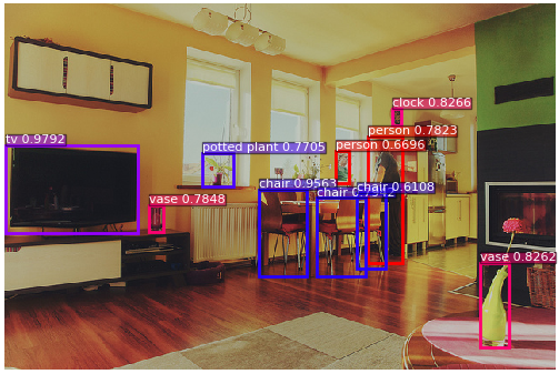
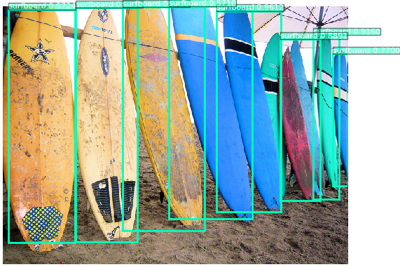
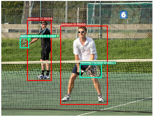
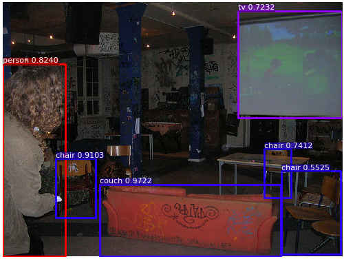
Visualization of infer result is shown as below:
<p align="center">
<img src="image/000000000139.png" height=300 width=400 hspace='10'/>
<img src="image/000000127517.png" height=300 width=400 hspace='10'/>
<img src="image/000000203864.png" height=300 width=400 hspace='10'/>
<img src="image/000000515077.png" height=300 width=400 hspace='10'/> <br />
YOLOv3 Visualization Examples
</p>