# Recommender System The source code of this tutorial is in [book/recommender_system](https://github.com/PaddlePaddle/book/tree/develop/05.recommender_system). For new users, please refer to [Running This Book](https://github.com/PaddlePaddle/book/blob/develop/README.md#running-the-book) . ## Background Introduction With the continuous development of network technology and the ever-expanding scale of e-commerce, the number and variety of goods grow rapidly and users need to spend a lot of time to find the goods they want to buy. This is information overload. In order to solve this problem, recommendation system came into being. The recommendation system is a subset of the Information Filtering System, which can be used in a range of areas such as movies, music, e-commerce, and Feed stream recommendations. The recommendation system discovers the user's personalized needs and interests by analyzing and mining user behaviors, and recommends information or products that may be of interest to the user. Unlike search engines, recommendation system do not require users to accurately describe their needs, but model their historical behavior to proactively provide information that meets user interests and needs. The GroupLens system \[[1](#references)\] introduced by the University of Minnesota in 1994 is generally considered to be a relatively independent research direction for the recommendation system. The system first proposed the idea of completing recommendation task based on collaborative filtering. After that, the collaborative filtering recommendation based on the model led the development of recommendation system for more than ten years. The traditional personalized recommendation system methods mainly include: - Collaborative Filtering Recommendation: This method is one of the most widely used technologies which requires the collection and analysis of users' historical behaviors, activities and preferences. It can usually be divided into two sub-categories: User-Based Recommendation \[[1](#references)\] and Item-Based Recommendation \[[2](#references)\]. A key advantage of this method is that it does not rely on the machine to analyze the content characteristics of the item, so it does not need to understand the item itself to accurately recommend complex items such as movies. However, the disadvantage is that there is a cold start problem for new users without any behavior. At the same time, there is also a sparsity problem caused by insufficient interaction data between users and commodities. It is worth mentioning that social network \[[3](#references)\] or geographic location and other context information can be integrated into collaborative filtering. - Content-Based Filtering Recommendation \[[4](#references)\] : This method uses the content description of the product to abstract meaningful features by calculating the similarity between the user's interest and the product description to make recommendations to users. The advantage is that it is simple and straightforward. It does not need to evaluate products based on the comments of users. Instead, it compares the product similarity by product attributes to recommend similar products to the users of interest. The disadvantage is that there is also a cold start problem for new users without any behavior. - Hybrid Recommendation \[[5](#references)\]: Use different inputs and techniques to jointly recommend items to complement each single recommendation technique. In recent years, deep learning has achieved great success in many fields. Both academia and industry are trying to apply deep learning to the field of recommendation systems. Deep learning has excellent ability to automatically extract features, can learn multi-level abstract feature representations, and learn heterogeneous or cross-domain content information, which can deal with the cold start problem \[[6](#references)\] of recommendation system to some extent. This tutorial focuses on the deep learning model of recommendation system and how to implement the model with PaddlePaddle. ## Result Demo We use a dataset containing user information, movie information, and movie ratings as a recommendation system. When we train the model, we only need to input the corresponding user ID and movie ID, we can get a matching score (range [0, 5], the higher the score is regarded as the greater interest), and then according to the recommendation of all movies sort the scores and recommend them to movies that may be of interest to the user. ``` Input movie_id: 1962 Input user_id: 1 Prediction Score is 4.25 ``` ## Model Overview In this chapter, we first introduce YouTube's video personalization recommendation system \[[7](#references)\], and then introduce the fusion recommendation model we implemented. ### YouTube's Deep Neural Network Personalized Recommendation System YouTube is the world's largest video uploading, sharing and discovery site, and the YouTube Personalized Recommendation System recommends personalized content from a growing library to more than 1 billion users. The entire system consists of two neural networks: a candidate generation network and a ranking network. The candidate generation network generates hundreds of candidates from a million-level video library, and the ranking network sorts the candidates and outputs the highest ranked tens of results. The system structure is shown in Figure 1:

Figure 1. YouTube personalized recommendation system structure

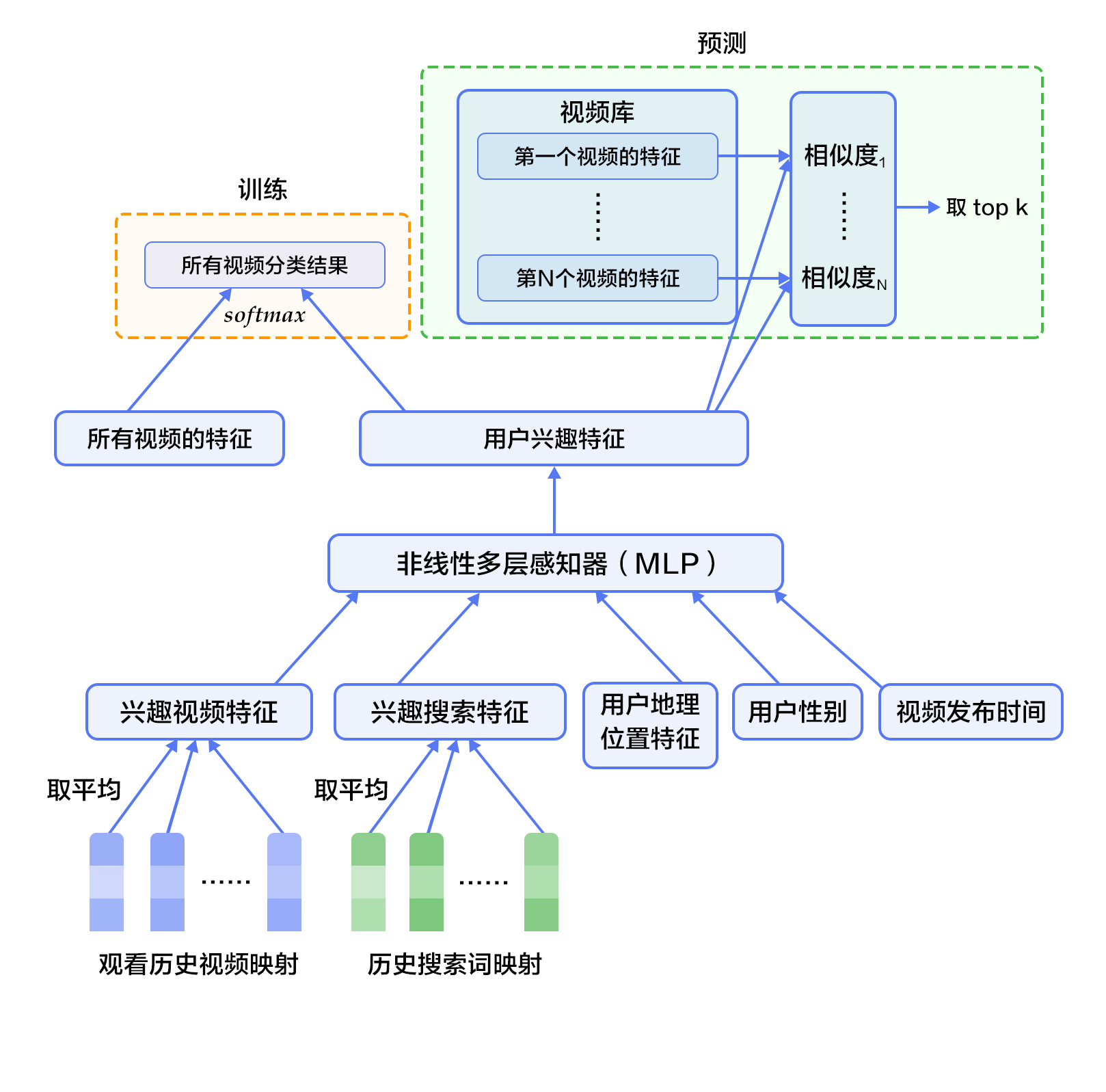
#### Candidate Generation Network The candidate generation network models the recommendation problem as a multi-class classification problem with a large number of categories. For a Youtube user, using its watching history (video ID), search tokens, demographic information (such as geographic location, user login device), binary features (such as gender, whether to log in), and continuous features (such as user age), etc., multi-classify all videos in the video library to obtain the classification result of each category (ie, the recommendation probability of each video), eventually outputting hundreds of videos with high probability. First, the historical information such as watching history and search token records are mapped to vectors and averaged to obtain a fixed length representation. At the same time, demographic characteristics are input to optimize the recommendation effect of new users, and the binary features and continuous features are normalized to the range [0, 1]. Next, put all the feature representations into a vector and input them to the non-linear multilayer perceptron (MLP, see [Identification Figures](https://github.com/PaddlePaddle/book/blob/develop/02.recognize_digits/README.md) tutorial). Finally, during training, the output of the MLP is classified by softmax. When predicting, the similarity of the user's comprehensive features (MLP output) to all videos' features is calculated, and the highest score of $k$ is obtained as the result of the candidate generation network. Figure 2 shows the candidate generation network structure.

Figure 2. Candidate generation network structure

For a user $U$, the formula for predicting whether the video $\omega$ that the user wants to watch at the moment is video $i$ is: $$P(\omega=i|u)=\frac{e^{v_{i}u}}{\sum_{j \in V}e^{v_{j}u}}$$ Where $u$ is the feature representation of the user $U$, $V$ is the video library collection, and $v_i$ is the feature representation of the $i$ video in the video library. $u$ and $v_i$ are vectors of equal length, and the dot product can be implemented by a fully connected layer. Considering that the number of categories in the softmax classification is very large, in order to ensure a certain computational efficiency: 1) in the training phase, use negative sample category sampling to reduce the number of actually calculated categories to thousands; 2) in the recommendation (prediction) phase, ignore the normalized calculation of softmax (does not affect the result), and simplifies the category scoring problem into the nearest neighbor search problem in the dot product space, then takes the nearest $k$ video of $u$ as a candidate for generation. #### Ranking Network The structure of the ranking network is similar to the candidate generation network, but its goal is to perform finer ranking of the candidates. Similar to the feature extraction method in traditional advertisement ranking, a large number of related features (such as video ID, last watching time, etc.) for video sorting are also constructed here. These features are treated similarly to the candidate generation network, except that at the top of the ranking network is a weighted logistic regression that scores all candidate videos and sorts them from high to low. Then, return to the user. ### Fusion recommendation model This section uses Convolutional Neural Networks to learn the representation of movie titles. The convolutional neural network for text and the fusion recommendation model are introduced in turn. #### Convolutional Neural Network (CNN) for text Convolutional neural networks are often used to deal with data of a grid-like topology. For example, an image can be viewed as a pixel of a two-dimensional grid, and a natural language can be viewed as a one-dimensional sequence of words. Convolutional neural networks can extract a variety of local features and combine them to obtain more advanced feature representations. Experiments show that convolutional neural networks can efficiently model image and text problems. The convolutional neural network is mainly composed of convolution and pooling operations, and its application and combination methods are flexible and varied. In this section we will explain the network as shown in Figure 3:

Figure 3. Convolutional neural network text classification model

Suppose the length of the sentence to be processed is $n$, where the word vector of the $i$ word is $x_i\in\mathbb{R}^k$, and $k$ is the dimension size. First, splicing the word vector: splicing each $h$ word to form a word window of size $h$, denoted as $x_{i:i+h-1}$, which represents the word sequence splicing of $x_{i}, x_{i+1}, \ldots, x_{i+h-1}$, where $i$ represents the position of the first word in the word window throughout the sentence, ranging from $1$ to $n-h+1$, $x_{i:i+h-1}\in\mathbb{R}^{hk}$. Second, perform a convolution operation: apply the convolution kernel $w\in\mathbb{R}^{hk}$ to the window $x_{i:i+h-1}$ containing $h$ words. , get the feature $c_i=f(w\cdot x_{i:i+h-1}+b)$, where $b\in\mathbb{R}$ is the bias and $f$ is the non Linear activation function, such as $sigmoid$. Apply the convolution kernel to all word windows ${x_{1:h}, x_{2:h+1},\ldots,x_{n-h+1:n}}$ in the sentence, producing a feature map: $$c=[c_1,c_2,\ldots,c_{n-h+1}], c \in \mathbb{R}^{n-h+1}$$ Next, using the max pooling over time for feature maps to obtain the feature $\hat c$, of the whole sentence corresponding to this convolution kernel, which is the maximum value of all elements in the feature map: $$\hat c=max(c)$$ #### Fusion recommendation model overview In the film personalized recommendation system that incorporates the recommendation model: 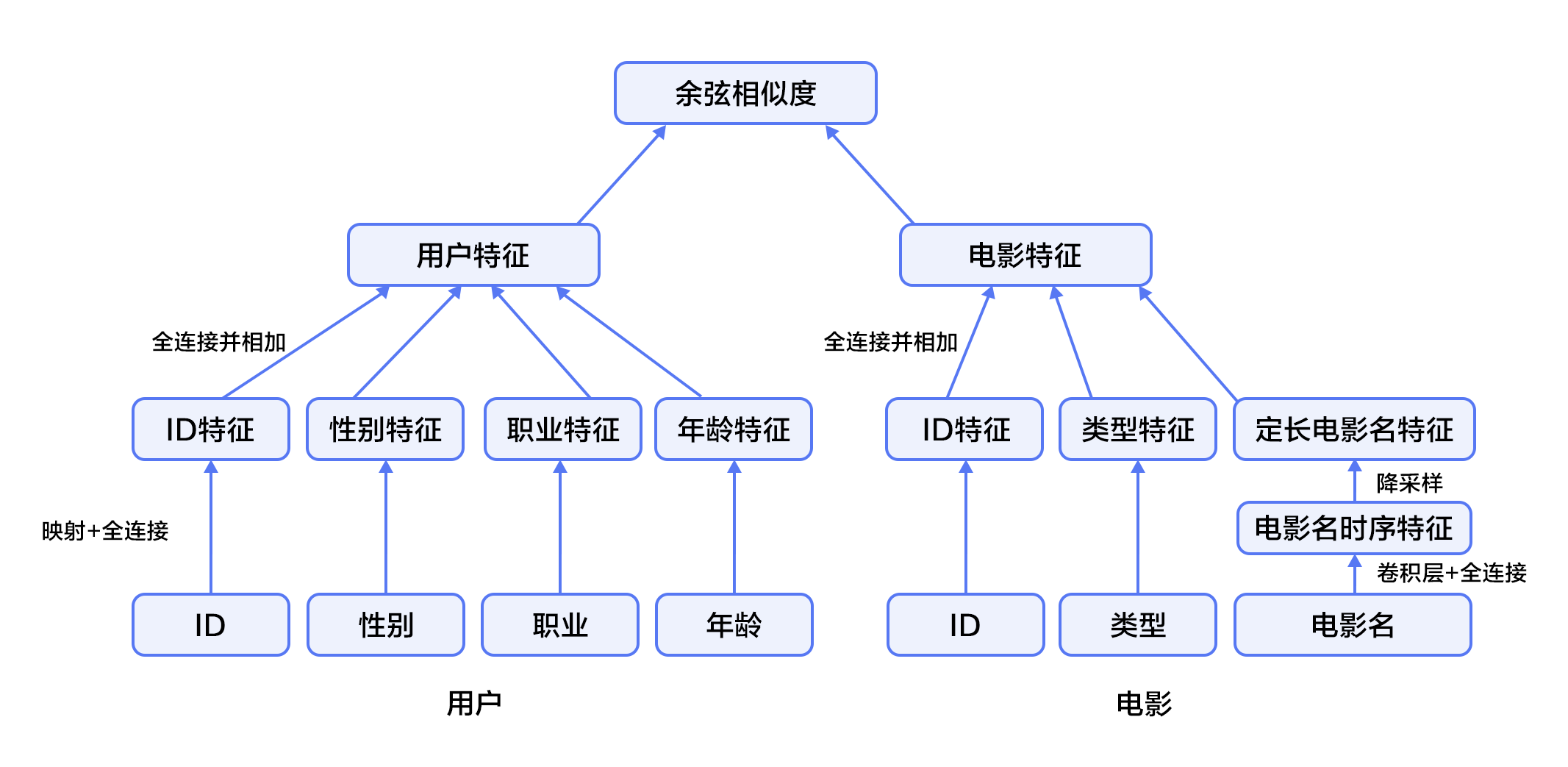1. First, take user features and movie features as input to the neural network, where: - The user features incorporate four attribute information: user ID, gender, occupation, and age. - The movie feature incorporate three attribute information: movie ID, movie type ID, and movie name. 2. For the user feature, map the user ID to a vector representation with a dimension size of 256, enter the fully connected layer, and do similar processing for the other three attributes. Then the feature representations of the four attributes are fully connected and added separately. 3. For movie features, the movie ID is processed in a manner similar to the user ID. The movie type ID is directly input into the fully connected layer in the form of a vector, and the movie name is represented by a fixed-length vector using a text convolutional neural network. The feature representations of the three attributes are then fully connected and added separately. 4. After obtaining the vector representation of the user and the movie, calculate the cosine similarity of them as the score of the personalized recommendation system. Finally, the square of the difference between the similarity score and the user's true score is used as the loss function of the regression model.

Figure 4. Fusion recommendation model

## Data Preparation ### Data Introduction and Download We take [MovieLens Million Dataset (ml-1m)](http://files.grouplens.org/datasets/movielens/ml-1m.zip) as an example. The ml-1m dataset contains 1,000,000 reviews of 4,000 movies by 6,000 users (scores ranging from 1 to 5, all integer), collected by the GroupLens Research lab. Paddle provides modules for automatically loading data in the API. The data module is `paddle.dataset.movielens` ```python from __future__ import print_function import paddle movie_info = paddle.dataset.movielens.movie_info() print(list(movie_info.values())[0]) ``` ```python # Run this block to show dataset's documentation # help(paddle.dataset.movielens) ``` The original data includes feature data of the movie, user's feature data, and the user's rating of the movie. For example, one of the movie features is: ```python movie_info = paddle.dataset.movielens.movie_info() print(list(movie_info.values())[0]) ``` This means that the movie id is 1, and the title is 《Toy Story》, which is divided into three categories. These three categories are animation, children, and comedy. ```python user_info = paddle.dataset.movielens.user_info() print(list(user_info.values())[0]) ``` This means that the user ID is 1, female, and younger than 18 years old. The occupation ID is 10. Among them, the age uses the following distribution * 1: "Under 18" * 18: "18-24" * 25: "25-34" * 35: "35-44" * 45: "45-49" * 50: "50-55" * 56: "56+" The occupation is selected from the following options: * 0: "other" or not specified * 1: "academic/educator" * 2: "artist" * 3: "clerical/admin" * 4: "college/grad student" * 5: "customer service" * 6: "doctor/health care" * 7: "executive/managerial" * 8: "farmer" * 9: "homemaker" * 10: "K-12 student" * 11: "lawyer" * 12: "programmer" * 13: "retired" * 14: "sales/marketing" * 15: "scientist" * 16: "self-employed" * 17: "technician/engineer" * 18: "tradesman/craftsman" * 19: "unemployed" * 20: "writer" For each training or test data, it is + + rating. For example, we get the first training data: ```python train_set_creator = paddle.dataset.movielens.train() train_sample = next(train_set_creator()) uid = train_sample[0] mov_id = train_sample[len(user_info[uid].value())] print("User %s rates Movie %s with Score %s"%(user_info[uid], movie_info[mov_id], train_sample[-1])) ``` User rates Movie with Score [5.0] That is, the user 1 evaluates the movie 1193 as 5 points. ## Configuration Instruction Below we begin to configure the model based on the form of the input data. First import the required library functions and define global variables. - IS_SPARSE: whether to use sparse update in embedding - PASS_NUM: number of epoch ```python import math import sys import numpy as np import paddle import paddle.fluid as fluid import paddle.fluid.layers as layers import paddle.fluid.nets as nets IS_SPARSE = True BATCH_SIZE = 256 PASS_NUM = 20 ``` Then define the model configuration for our user feature synthesis model ```python def get_usr_combined_features(): """network definition for user part""" USR_DICT_SIZE = paddle.dataset.movielens.max_user_id() + 1 uid = fluid.data(name='user_id', shape=[-1], dtype='int64') usr_emb = fluid.embedding( input=uid, dtype='float32', size=[USR_DICT_SIZE, 32], param_attr='user_table', is_sparse=IS_SPARSE) usr_fc = layers.fc(input=usr_emb, size=32) USR_GENDER_DICT_SIZE = 2 usr_gender_id = fluid.data(name='gender_id', shape=[-1], dtype='int64') usr_gender_emb = fluid.embedding( input=usr_gender_id, size=[USR_GENDER_DICT_SIZE, 16], param_attr='gender_table', is_sparse=IS_SPARSE) usr_gender_fc = layers.fc(input=usr_gender_emb, size=16) USR_AGE_DICT_SIZE = len(paddle.dataset.movielens.age_table) usr_age_id = fluid.data(name='age_id', shape=[-1], dtype="int64") usr_age_emb = fluid.embedding( input=usr_age_id, size=[USR_AGE_DICT_SIZE, 16], is_sparse=IS_SPARSE, param_attr='age_table') usr_age_fc = layers.fc(input=usr_age_emb, size=16) USR_JOB_DICT_SIZE = paddle.dataset.movielens.max_job_id() + 1 usr_job_id = fluid.data(name='job_id', shape=[-1], dtype="int64") usr_job_emb = fluid.embedding( input=usr_job_id, size=[USR_JOB_DICT_SIZE, 16], param_attr='job_table', is_sparse=IS_SPARSE) usr_job_fc = layers.fc(input=usr_job_emb, size=16) concat_embed = layers.concat( input=[usr_fc, usr_gender_fc, usr_age_fc, usr_job_fc], axis=1) usr_combined_features = layers.fc(input=concat_embed, size=200, act="tanh") return usr_combined_features ``` As shown in the code above, for each user, we enter a 4-dimensional feature. This includes user_id, gender_id, age_id, job_id. These dimensional features are simple integer values. In order to facilitate the subsequent neural network processing of these features, we use the language model in NLP to transform these discrete integer values ​​into embedding. And form them into usr_emb, usr_gender_emb, usr_age_emb, usr_job_emb, respectively. Then, we enter all the user features into a fully connected layer(fc). Combine all features into one 200-dimension feature. Furthermore, we make a similar transformation for each movie feature, the network configuration is: ```python def get_mov_combined_features(): """network definition for item(movie) part""" MOV_DICT_SIZE = paddle.dataset.movielens.max_movie_id() + 1 mov_id = fluid.data(name='movie_id', shape=[-1], dtype='int64') mov_emb = fluid.embedding( input=mov_id, dtype='float32', size=[MOV_DICT_SIZE, 32], param_attr='movie_table', is_sparse=IS_SPARSE) mov_fc = layers.fc(input=mov_emb, size=32) CATEGORY_DICT_SIZE = len(paddle.dataset.movielens.movie_categories()) category_id = fluid.data( name='category_id', shape=[-1], dtype='int64', lod_level=1) mov_categories_emb = fluid.embedding( input=category_id, size=[CATEGORY_DICT_SIZE, 32], is_sparse=IS_SPARSE) mov_categories_hidden = layers.sequence_pool( input=mov_categories_emb, pool_type="sum") MOV_TITLE_DICT_SIZE = len(paddle.dataset.movielens.get_movie_title_dict()) mov_title_id = fluid.data( name='movie_title', shape=[-1], dtype='int64', lod_level=1) mov_title_emb = fluid.embedding( input=mov_title_id, size=[MOV_TITLE_DICT_SIZE, 32], is_sparse=IS_SPARSE) mov_title_conv = nets.sequence_conv_pool( input=mov_title_emb, num_filters=32, filter_size=3, act="tanh", pool_type="sum") concat_embed = layers.concat( input=[mov_fc, mov_categories_hidden, mov_title_conv], axis=1) mov_combined_features = layers.fc(input=concat_embed, size=200, act="tanh") return mov_combined_features ``` The title of a movie is a sequence of integers, and the integer represents the subscript of the word in the index sequence. This sequence is sent to the `sequence_conv_pool` layer, which uses convolution and pooling on the time dimension. Because of this, the output will be fixed length, although the length of the input sequence will vary. Finally, we define an `inference_program` to calculate the similarity between user features and movie features using cosine similarity. ```python def inference_program(): """the combined network""" usr_combined_features = get_usr_combined_features() mov_combined_features = get_mov_combined_features() inference = layers.cos_sim(X=usr_combined_features, Y=mov_combined_features) scale_infer = layers.scale(x=inference, scale=5.0) return scale_infer ``` Furthermore, we define a `train_program` to use the result computed by `inference_program`, and calculate the error with the help of the tag data. We also define an `optimizer_func` to define the optimizer. ```python def train_program(): """define the cost function""" scale_infer = inference_program() label = fluid.data(name='score', shape=[-1, 1], dtype='float32') square_cost = layers.square_error_cost(input=scale_infer, label=label) avg_cost = layers.mean(square_cost) return [avg_cost, scale_infer] def optimizer_func(): return fluid.optimizer.SGD(learning_rate=0.2) ``` ## Training Model ### Defining the training environment Define your training environment and specify whether the training takes place on CPU or GPU. ```python use_cuda = False place = fluid.CUDAPlace(0) if use_cuda else fluid.CPUPlace() ``` ### Defining the data provider The next step is to define a data provider for training and testing. The provider reads in a data of size `BATCH_SIZE`. `paddle.dataset.movielens.train` will provide a data of size `BATCH_SIZE` after each scribbling, and the size of the out-of-order is the cache size `buf_size`. ```python train_reader = fluid.io.batch( fluid.io.shuffle( paddle.dataset.movielens.train(), buf_size=8192), batch_size=BATCH_SIZE) test_reader = fluid.io.batch( paddle.dataset.movielens.test(), batch_size=BATCH_SIZE) ``` ### Constructing a training process (trainer) We have constructed a training process here, including training optimization functions. ### Provide data `feed_order` is used to define the mapping between each generated data and `paddle.layer.data`. For example, the data in the first column generated by `movielens.train` corresponds to the feature `user_id`. ```python feed_order = [ 'user_id', 'gender_id', 'age_id', 'job_id', 'movie_id', 'category_id', 'movie_title', 'score' ] ``` ### Building training programs and testing programs The training program and the test program are separately constructed, and the training optimizer is imported. ```python main_program = fluid.default_main_program() star_program = fluid.default_startup_program() [avg_cost, scale_infer] = train_program() test_program = main_program.clone(for_test=True) sgd_optimizer = optimizer_func() sgd_optimizer.minimize(avg_cost) exe = fluid.Executor(place) def train_test(program, reader): count = 0 feed_var_list = [ program.global_block().var(var_name) for var_name in feed_order ] feeder_test = fluid.DataFeeder( feed_list=feed_var_list, place=place) test_exe = fluid.Executor(place) accumulated = 0 for test_data in reader(): avg_cost_np = test_exe.run(program=program, feed=feeder_test.feed(test_data), fetch_list=[avg_cost]) accumulated += avg_cost_np[0] count += 1 return accumulated / count ``` ### Build a training main loop and start training We perform the training cycle according to the training cycle number (`PASS_NUM`) defined above and some other parameters, and perform a test every time. When the test result is good enough, we exit the training and save the trained parameters. ```python # Specify the directory path to save the parameters params_dirname = "recommender_system.inference.model" from paddle.utils.plot import Ploter train_prompt = "Train cost" test_prompt = "Test cost" plot_cost = Ploter(train_prompt, test_prompt) def train_loop(): feed_list = [ main_program.global_block().var(var_name) for var_name in feed_order ] feeder = fluid.DataFeeder(feed_list, place) exe.run(star_program) for pass_id in range(PASS_NUM): for batch_id, data in enumerate(train_reader()): # train a mini-batch outs = exe.run(program=main_program, feed=feeder.feed(data), fetch_list=[avg_cost]) out = np.array(outs[0]) # get test avg_cost test_avg_cost = train_test(test_program, test_reader) plot_cost.append(train_prompt, batch_id, outs[0]) plot_cost.append(test_prompt, batch_id, test_avg_cost) plot_cost.plot() if batch_id == 20: if params_dirname is not None: fluid.io.save_inference_model(params_dirname, [ "user_id", "gender_id", "age_id", "job_id", "movie_id", "category_id", "movie_title" ], [scale_infer], exe) return print('EpochID {0}, BatchID {1}, Test Loss {2:0.2}'.format( pass_id + 1, batch_id + 1, float(test_avg_cost))) if math.isnan(float(out[0])): sys.exit("got NaN loss, training failed.") ``` Start training ```python train_loop() ``` ## Model Application ### Generate test data Use the API of create_lod_tensor(data, lod, place) to generate the tensor of the detail level. `data` is a sequence, and each element is a sequence of index numbers. `lod` is the detail level's information, corresponding to `data`. For example, data = [[10, 2, 3], [2, 3]] means that it contains two sequences of lengths 3 and 2. Correspondingly lod = [[3, 2]], which indicates that it contains a layer of detail information, meaning that `data` has two sequences, lengths of 3 and 2. In this prediction example, we try to predict the score given by user with ID1 for the movie 'Hunchback of Notre Dame'. ```python infer_movie_id = 783 infer_movie_name = paddle.dataset.movielens.movie_info()[infer_movie_id].title user_id = np.array([1]).astype("int64").reshape(-1) gender_id = np.array([1]).astype("int64").reshape(-1) age_id = np.array([0]).astype("int64").reshape(-1) job_id = np.array([10]).astype("int64").reshape(-1) movie_id = np.array([783]).astype("int64").reshape(-1) # Hunchback of Notre Dame category_id = fluid.create_lod_tensor(np.array([10, 8, 9], dtype='int64'), [[3]], place) # Animation, Children's, Musical movie_title = fluid.create_lod_tensor(np.array([1069, 4140, 2923, 710, 988], dtype='int64'), [[5]], place) # 'hunchback','of','notre','dame','the' ``` ### Building the prediction process and testing Similar to the training process, we need to build a prediction process, where `params_dirname` is the address used to store the various parameters in the training process. ```python place = fluid.CUDAPlace(0) if use_cuda else fluid.CPUPlace() exe = fluid.Executor(place) inference_scope = fluid.core.Scope() ``` ### Testing Now we can make predictions. The `feed_order` we provide should be consistent with the training process. ```python with fluid.scope_guard(inference_scope): [inferencer, feed_target_names, fetch_targets] = fluid.io.load_inference_model(params_dirname, exe) results = exe.run(inferencer, feed={ 'user_id': user_id, 'gender_id': gender_id, 'age_id': age_id, 'job_id': job_id, 'movie_id': movie_id, 'category_id': category_id, 'movie_title': movie_title }, fetch_list=fetch_targets, return_numpy=False) predict_rating = np.array(results[0]) print("Predict Rating of user id 1 on movie \"" + infer_movie_name + "\" is " + str(predict_rating[0][0])) print("Actual Rating of user id 1 on movie \"" + infer_movie_name + "\" is 4.") ``` ## Summary This chapter introduced the traditional personalized recommendation system method and YouTube's deep neural network personalized recommendation system. It further took movie recommendation as an example, and used PaddlePaddle to train a personalized recommendation neural network model. The personalized recommendation system covers almost all aspects of e-commerce systems, social networks, advertising recommendations, search engines, etc. Deep learning technologies have played an important role in image processing, natural language processing, etc., and will also prevail in personalized recommendation systems. ## References 1. P. Resnick, N. Iacovou, etc. “[GroupLens: An Open Architecture for Collaborative Filtering of Netnews](http://ccs.mit.edu/papers/CCSWP165.html)”, Proceedings of ACM Conference on Computer Supported Cooperative Work, CSCW 1994. pp.175-186. 2. Sarwar, Badrul, et al. "[Item-based collaborative filtering recommendation algorithms.](http://files.grouplens.org/papers/www10_sarwar.pdf)" *Proceedings of the 10th international conference on World Wide Web*. ACM, 2001. 3. Kautz, Henry, Bart Selman, and Mehul Shah. "[Referral Web: combining social networks and collaborative filtering.](http://www.cs.cornell.edu/selman/papers/pdf/97.cacm.refweb.pdf)" Communications of the ACM 40.3 (1997): 63-65. APA 4. [Peter Brusilovsky](https://en.wikipedia.org/wiki/Peter_Brusilovsky) (2007). *The Adaptive Web*. p. 325. 5. Robin Burke , [Hybrid Web recommendation systems](http://citeseerx.ist.psu.edu/viewdoc/download?doi=10.1.1.435.7538&rep=rep1&type=pdf), pp. 377-408, The Adaptive Web, Peter Brusilovsky, Alfred Kobsa, Wolfgang Nejdl (Ed.), Lecture Notes in Computer Science, Springer-Verlag, Berlin, Germany, Lecture Notes in Computer Science, Vol. 4321, May 2007, 978-3-540-72078-2. 6. Yuan, Jianbo, et al. ["Solving Cold-Start Problem in Large-scale Recommendation Engines: A Deep Learning Approach."](https://arxiv.org/pdf/1611.05480v1.pdf) *arXiv preprint arXiv:1611.05480* (2016). 7. Covington P, Adams J, Sargin E. [Deep neural networks for youtube recommendations](https://static.googleusercontent.com/media/research.google.com/zh-CN//pubs/archive/45530.pdf)[C]//Proceedings of the 10th ACM Conference on recommendation systems. ACM, 2016: 191-198.

This tutorial is contributed by PaddlePaddle, and licensed under a Creative Commons Attribution-ShareAlike 4.0 International License.