# Machine Translation Source code of this tutorial is in [book/machine_translation](https://github.com/PaddlePaddle/book/tree/develop/08.machine_translation). For users new to Paddle book, please refer to [the user guide of Book Documentation](https://github.com/PaddlePaddle/book/blob/develop/README.cn.md#run_the_book). ## Background Machine translation is to translate different languages with computer. The language to be translated is usually called source language, and the language representing the result of translation is called target language. Machine translation is the process of transformation from source language to target language, which is an important research assignment of Natural Language Processing. Machine translation systems at early age were mostly rule-based translation system, which needs linguists make transformation rule between two languages and then input these rules into computer. This method requires proficient professional linguistic background, but it is hard to cover all rules of a language, let it alone two or more languages. Therefore, the major challenge of traditional machine translation method is the impossibility of a completest set of rules\[[1](#References)\]. To solve the problem mentioned above, Statistical Machine Translation technology emerged afterwards. For Statistical Machine Translation, transformation rules are automatically learned from a large scale corpus instead of handcrafted rule. So it tackles with the limit of obtaining knowledge in rule-based machine translation systems. However, it still faces certain challenges: 1. man-made feature can never cover all language phenomena. 2. it is hard to use global feature. 3. it depends on many pre-processing parts, such as Word Alignment, Tokenization, Rule Extraction, Parsing. Errors accumulated by those parts will have a great influence on translation. In recent years, Deep Learning technology proposes new solutions to overcome the bottleneck. Two methods for machine translation are realized with the aid of deep learning. 1. Based on the framework of statistical machine translation system, the neural network is in place to improve core parts, such as language model, reordering model and so on (See the left part in figure One). 2. Abandoning the framework of statistical machine translation system, it directly uses neural network to transform source language to target language, which is End-to-End Neural Machine Translation (See right part in figure One), NMT model in short.

Figure One. Neural Network Machine Translation System
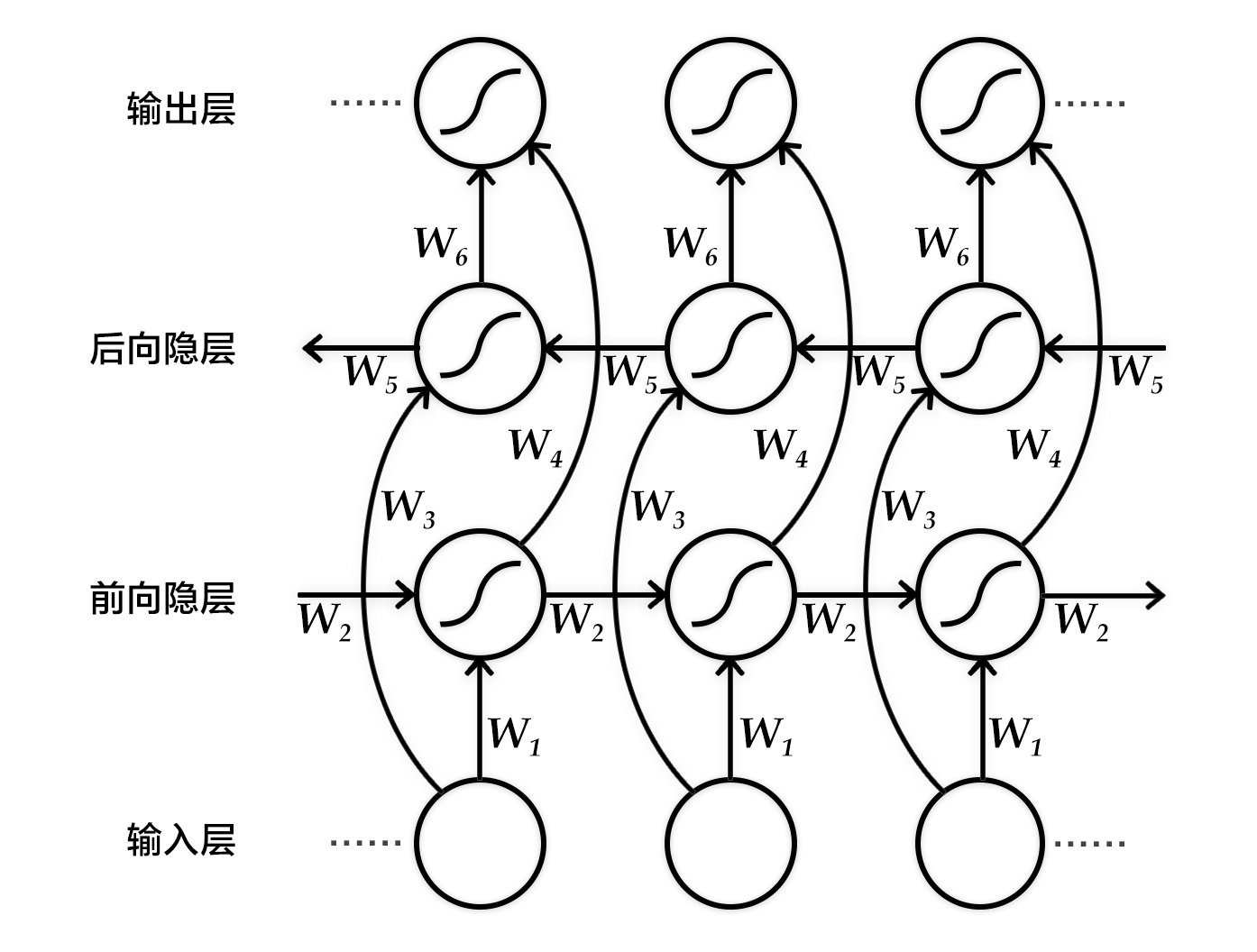
In the following parts, we'll guide you through NMT model and its hands-on implementation in PaddlePaddle ## Result Demo Take Chinese to English translation model as an example. For a trained model, if input the following tokenized Chinese sentence : ```text 这些 是 希望 的 曙光 和 解脱 的 迹象 . ``` If it sets the entries of translation result ( e.t. the width of [beam search algorithm](#beam search algorithm)) as 3, the generated English sentence is as follows: ```text 0 -5.36816 These are signs of hope and relief . 1 -6.23177 These are the light of hope and relief . 2 -7.7914 These are the light of hope and the relief of hope . ``` - The first column to the left is the serial numbers of generated sentences. The second column from left is scores of the sentences in descending order, in which higher score is better. The third column contains the generated English sentences. - In addition, there are two special marks. One is ``, indicating the end of a sentence and another one is ``, representing unknown word, which have never appeared in dictionary. ## Exploration of Models In this section, let's scrutinize Bi-directional Recurrent Neural Network, typical Encoder-Decoder structure in NMT model and beam search algorithm. ### Bi-directional Recurrent Neural Network We have introduced a bi-directional recurrent neural network in the chapter [label_semantic_roles](https://github.com/PaddlePaddle/book/blob/develop/07.label_semantic_roles/README.md). Here we introduce another network proposed by Bengio team in thesis \[[2](#References),[4](#References)\] The aim of this network is to input a sequence and get its features at each time step. Specifically, fixed-length vector is incorporated to represent contextual semantic information for each time step in the output. To be concrete, the Bi-directional recurrent neural network sequentially processes the input sequences in time dimension in sequential order or in reverse order, i.e., forward and backward. And the output of RNN at each time step are concatenated to be the final output layer. Hereby the output node of each time step contains complete past and future context information of current time step of input sequence. The figure below shows a bi-directional recurrent neural network expanded by time step. The network consists of a forward and a backward RNN with six weight matrices: a weight matrix ($W_1, W_3$) from input layer to the forward and backward hidden layers, and a weight matrix ($W_2, W_5$) from a hidden layer to itself (self-loop), the weight matrix from the forward hidden layer and the backward hidden layer to the output layer ($W_4, W_6$). Note that there is no connection between the forward hidden layer and the backward hidden layer.

Figure 2. Bi-directional Recurrent Neural Network expanded by time step.
### Encoder-Decoder Structure The Encoder-Decoder\[[2](#References)\] structure helps transform a source sequence with arbitrary length to another target sequence with arbitrary length. In the encoding phase, it encodes the entire source sequence into a vector. And in the decoding phase, it decodes the entire target sequence by maximizing the predicted sequence probability. The encoding and decoding process is usually implemented by RNN.

Figure 3. Encoder-Decoder Frame
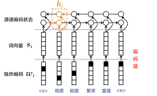
#### Encoder Encoding can be done in 3 steps: 1.One-hot vector : each word $x_i$ of the source language sentence $x=\left \{ x_1,x_2,...,x_T \right \}$ is represented as a column vector $w_i\epsilon \left \{ 0,1 \right \}^{\left | V \right |},i=1,2,...,T$. The dimension of this vector $w_i$ is the same as the vocabulary size $\left | V \right |$, and there is only one dimension with a value of 1 (the position corresponds to the position of the word in the vocabulary), and the rest are all zero. 2.Word vector mapped to low-dimensional semantic space: one-hot vector indicates that there are two problems: 1. the dimension of generated vector is often large, which is easy to cause dimension disaster. 2. it is difficult to characterize the relationship between words and words (such as semantical similarity, that is, the semantics cannot be expressed well.) Therefore, one-hot vector needs to be mapped to a low-dimensional semantic space, represented by a dense vector(called a word vector) with fixed dimensions . The mapping matrix is $C\epsilon R^{K\times \left | V \right |}$, with $s_i=Cw_i$ representing the word vector of the $i$ word, $K$ representing the dimension of vector. 3.Encode a source language word sequence with RNN: The calculation for this process is $h_i=\varnothing _\theta \left ( h_{i-1}, s_i \right )$, where $h_0$ is an all-zero vector. $\varnothing _\theta$ is a non-linear activation function, and the result $\mathbf{h}=\left \{ h_1,..., h_T \right \}$ is the state code sequence of source language $T$ words read by RNN respectively. The vector representation of the entire sentence can use $\mathbf{h}$ in the state code of the last time step $T$, or use the pooling result in the time dimension. Step 3 can also use bi-directional recurrent neural network to implement more complex sentence-coded representation, which can be implemented with bi-directional GRU. The forward GRU sequentially encodes the source language word in the order of the word sequence $(x_1, x_2,..., x_T)$, and obtains a series of hidden layer states $(\overrightarrow{h_1},\overrightarrow{h_2},. ..,\overrightarrow{h_T})$. Similarly, the backward GRU encodes the source language word in the order of $(x_T,x_{T-1},...,x_1)$, resulting in $(\overleftarrow{h_1},\overleftarrow{h_2},. ..,\overleftarrow{h_T})$. Finally, for the word $x_i$, the hidden layer state is obtained by jointing the two GRUs, namely $h_i=\left [ \overrightarrow{h_i^T},\overleftarrow{h_i^T} \right ]^{T} $.

Figure 4. Use bi-directional GRU encoder
#### Decoder During the training of machine translation tasks, the goal of in decode period is to maximize the probability of the next correct target language word. The idea is: 1.At each time, according to the encoding information of the source language sentence (also called context vector) $c$, the $i$th word $u_i$ of the real target language sequence and the hidden layer state $z_i $ of RNN at $i$th time, it calculates the next hidden layer state $z_{i+1}$. The formula is as follows: $$z_{i+1}=\phi_{\theta '} \left ( c,u_i,z_i \right )$$ Where $\phi _{\theta '}$ is a nonlinear activation function; $c$ is the context vector of the source language sentence, if the attention mechanism is not used and the output of [encoder](#encoder) is the last element after the source language sentence is encoded, you can define $c=h_T$; $u_i$ is the $i$th word of the target language sequence, and $u_0$ is the start tag `` of the target language sequence, indicating the start of decoding; $z_i$ is the hidden layer state of the RNN at $i$th time, and $z_0$ is an all-zero vector. 2.Normalize $z_{i+1}$ by `softmax` to get the probability distribution $p_{i+1}$ of the $i+1$th word of the target language sequence. The probability distribution formula is as follows: $$p\left ( u_{i+1}|u_{<i+1},\mathbf{x} \right )=softmax(W_sz_{i+1}+b_z)$$ Where $W_sz_{i+1}+b_z$ scores each possible output word and normalizes with softmax to get the probability $p_{i+1}$ of $i+1$th word. 3.Calculate the cost according to $p_{i+1}$ and $u_{i+1}$. 4.Repeat steps 1~3 until all words in the target language sequence have been processed. The process of generating machine translation tasks, in general, is to translate source language sentences based on pre-trained model. The decode period in the generation process is different from the training process above. For details, please refer to [Beam Search Algorithm](#Beam Search Algorithm). ### Beam Search Algorithm Beam Search ([beam search](http://en.wikipedia.org/wiki/Beam_search)) is a heuristic graph search algorithm for searching the graph or tree for the optimal extended nodes in a finite set, usually used in systems with very large solution space (such as machine translation, speech recognition), for that the memory can't fit all the unfolded solutions in the graph or tree. If you want to translate "`Hello`" in the machine translation task, even if there are only 3 words (``, ``, `hello`) in the target language dictionary, it is possible generate infinite sentences (the number of occurrences of `hello` is uncertain). In order to find better translation results, we can use beam search algorithm. The beam search algorithm uses a breadth-first strategy to build a search tree. At each level of the tree, the nodes are sorted according to the heuristic cost (in this tutorial, the sum of the log probabilities of the generated words), and then only the predetermined number of nodes (commonly referred to in the literature as beam width, beam size, 柱宽度, etc.). Only these nodes will continue to expand in the next layer, and other nodes will be cut off, that is, the nodes with higher quality are retained, and the nodes with poor quality are pruned. Therefore, the space and time occupied by the search are greatly reduced, but the disadvantage is that there is no guarantee that an optimal solution will be obtained. In the decode period of using beam search algorithm, the goal is to maximize the probability of generated sequence. The idea is: 1.At each time, the next hidden layer state $z_{i+1}$ is calculated according to the encoding information $c$ of the source language sentence, the generated $i$th target language sequence words $u_i$, and the hidden layer state $z_i$ of RNN at $i$th time. 2.Normalize $z_{i+1}$ by `softmax` to get the probability distribution $p_{i+1}$ of the $i+1$th words of the target language sequence. 3.The word $u_{i+1}$ is sampled according to $p_{i+1}$. 4.Repeat steps 1~3 until you get the sentence end tag `` or exceed the maximum generation length of the sentence. Note: The formula for $z_{i+1}$ and $p_{i+1}$ is the same as in [Decoder](#Decoder). And since each step of the generation is implemented by the greedy method, it is not guaranteed to obtain the global optimal solution. ## Data Preparation This tutorial uses [bitexts(after selection)] in the [WMT-14](http://www-lium.univ-lemans.fr/~schwenk/cslm_joint_paper/) dataset (http://www-lium.univ- Lemans.fr/~schwenk/cslm_joint_paper/data/bitexts.tgz) as a training set, [dev+test data](http://www-lium.univ-lemans.fr/~schwenk/cslm_joint_paper/data/dev+test.tgz) as a test set and generated set. ### Data Pre-processing It contains two steps in pre-processing: -Merge parallel corpora files from source language to target language into one file: -Merge every `XXX.src` and `XXX.trg` into one file as `XXX`. -Content in $i$th row of `XXX` is the connection of $i$th row of `XXX.src` with $i$th row of `XXX.trg`, which is divided by '\t'. -Create source language dictionary and target language dictionary of train data. There are **DICTSIZE** words in each dictionary, including: (DICTSIZE - 3) words with highest frequency in the corpus, and 3 special symbols `` (the beginning of the sequence), `` ( the end of the sequence) and `` (unknown word). ### Sample Data Because the data volume of the complete data set is large, in order to verify the training process, the PaddlePaddle interface paddle.data set.wmt14 provides a pre-processed [smaller scale dataset](http://paddlepaddle.bj.bcebos.com/demo/wmt_shrinked_data/wmt14.tgz) by default . In the data set, there are 193,319 training data, 6003 test data, and a dictionary with length of 30,000. Due to the limit of data size, the effects of models trained with this dataset are not guaranteed. ## Model Configuration Next we start configuring model according to input data. First we import necessary library functions and define global variables. ```python from __future__ import print_function import contextlib import numpy as np import paddle import paddle.fluid as fluid import paddle.fluid.framework as framework import paddle.fluid.layers as pd from paddle.fluid.executor import Executor from functools import partial import os try: from paddle.fluid.contrib.trainer import * from paddle.fluid.contrib.inferencer import * except ImportError: print( "In the fluid 1.0, the trainer and inferencer are moving to paddle.fluid.contrib", file=sys.stderr) from paddle.fluid.trainer import * from paddle.fluid.inferencer import * dict_size = 30000 # dictionary dimension source_dict_dim = target_dict_dim = dict_size # source/target language dictionary dimension hidden_dim = 32 # size of hidden layer in encoder word_dim = 16 # dimension of word vector batch_size = 2 # the number of samples in batch max_length = 8 # the maximum length of generated sentence beam_size = 2 # width of beam decoder_size = hidden_dim # size of hidden layer in decoder ``` Then the frame of encoder is implemented as follows: ```python def encoder(is_sparse): # define input data id of source language src_word_id = pd.data( name="src_word_id", shape=[1], dtype='int64', lod_level=1) # reflect encode above on the word vector of low-dimension language space. src_embedding = pd.embedding( input=src_word_id, size=[dict_size, word_dim], dtype='float32', is_sparse=is_sparse, param_attr=fluid.ParamAttr(name='vemb')) # LSTM layer:fc + dynamic_lstm fc1 = pd.fc(input=src_embedding, size=hidden_dim * 4, act='tanh') lstm_hidden0, lstm_0 = pd.dynamic_lstm(input=fc1, size=hidden_dim * 4) # Fetch the final state after the sequence encode of source language encoder_out = pd.sequence_last_step(input=lstm_hidden0) return encoder_out ``` Then implement decoder in training mode: ```python def train_decoder(context, is_sparse): # Define input data of sequence id of target language and reflect it on word vector of low-dimension language space trg_language_word = pd.data( name="target_language_word", shape=[1], dtype='int64', lod_level=1) trg_embedding = pd.embedding( input=trg_language_word, size=[dict_size, word_dim], dtype='float32', is_sparse=is_sparse, param_attr=fluid.ParamAttr(name='vemb')) rnn = pd.DynamicRNN() with rnn.block(): # use DynamicRNN to define computation at each step # Fetch input word vector of target language at present step current_word = rnn.step_input(trg_embedding) # obtain state of hidden layer pre_state = rnn.memory(init=context) # computing unit of decoder: single-layer forward network current_state = pd.fc(input=[current_word, pre_state], size=decoder_size, act='tanh') # compute predicting probability of nomarlized word current_score = pd.fc(input=current_state, size=target_dict_dim, act='softmax') # update hidden layer of RNN rnn.update_memory(pre_state, current_state) # output predicted probability rnn.output(current_score) return rnn() ``` implement decoder in inference mode ```python def decode(context, is_sparse): init_state = context # define counter variable in the decoding array_len = pd.fill_constant(shape=[1], dtype='int64', value=max_length) counter = pd.zeros(shape=[1], dtype='int64', force_cpu=True) # define tensor array to save content at each time step, and write initial id, score and state state_array = pd.create_array('float32') pd.array_write(init_state, array=state_array, i=counter) ids_array = pd.create_array('int64') scores_array = pd.create_array('float32') init_ids = pd.data(name="init_ids", shape=[1], dtype="int64", lod_level=2) init_scores = pd.data( name="init_scores", shape=[1], dtype="float32", lod_level=2) pd.array_write(init_ids, array=ids_array, i=counter) pd.array_write(init_scores, array=scores_array, i=counter) # define conditional variable to stop loop cond = pd.less_than(x=counter, y=array_len) # define while_op while_op = pd.While(cond=cond) with while_op.block(): # define the computing of each step # obtain input at present step of decoder, including id chosen at previous step, corresponding score and state at previous step. pre_ids = pd.array_read(array=ids_array, i=counter) pre_state = pd.array_read(array=state_array, i=counter) pre_score = pd.array_read(array=scores_array, i=counter) # update input state as state correspondent with id chosen at previous step pre_state_expanded = pd.sequence_expand(pre_state, pre_score) # computing logic of decoder under the same train mode, including input vector and computing unit of decoder # compute predicting probability of normalized word pre_ids_emb = pd.embedding( input=pre_ids, size=[dict_size, word_dim], dtype='float32', is_sparse=is_sparse) current_state = pd.fc(input=[pre_state_expanded, pre_ids_emb], size=decoder_size, act='tanh') current_state_with_lod = pd.lod_reset(x=current_state, y=pre_score) current_score = pd.fc(input=current_state_with_lod, size=target_dict_dim, act='softmax') topk_scores, topk_indices = pd.topk(current_score, k=beam_size) # compute accumulated score and perform beam search accu_scores = pd.elementwise_add( x=pd.log(topk_scores), y=pd.reshape(pre_score, shape=[-1]), axis=0) selected_ids, selected_scores = pd.beam_search( pre_ids, pre_score, topk_indices, accu_scores, beam_size, end_id=10, level=0) pd.increment(x=counter, value=1, in_place=True) # write search result and corresponding hidden layer into tensor array pd.array_write(current_state, array=state_array, i=counter) pd.array_write(selected_ids, array=ids_array, i=counter) pd.array_write(selected_scores, array=scores_array, i=counter) # update condition to stop loop length_cond = pd.less_than(x=counter, y=array_len) finish_cond = pd.logical_not(pd.is_empty(x=selected_ids)) pd.logical_and(x=length_cond, y=finish_cond, out=cond) translation_ids, translation_scores = pd.beam_search_decode( ids=ids_array, scores=scores_array, beam_size=beam_size, end_id=10) return translation_ids, translation_scores ``` Furthermore, we define a `train_program` to use result computed by `inference_program` and compute error with the help of marked data. We also define an `optimizer_func` to define optimizer. ```python def train_program(is_sparse): context = encoder(is_sparse) rnn_out = train_decoder(context, is_sparse) label = pd.data( name="target_language_next_word", shape=[1], dtype='int64', lod_level=1) cost = pd.cross_entropy(input=rnn_out, label=label) avg_cost = pd.mean(cost) return avg_cost def optimizer_func(): return fluid.optimizer.Adagrad( learning_rate=1e-4, regularization=fluid.regularizer.L2DecayRegularizer( regularization_coeff=0.1)) ``` ## Train Model ### Define Training Environment Define your training environment and define the train executed on CPU or on GPU. ```python use_cuda = False place = fluid.CUDAPlace(0) if use_cuda else fluid.CPUPlace() ``` ### Define Data Provider The next step is to define data provider for train and test. Data Provider read data with size of `BATCH_SIZE` `paddle.dataset.wmt.train` will provide data with size of `BATCH_SIZE` after reordering every time. The size of reordering is `buf_size`. ```python train_reader = paddle.batch( paddle.reader.shuffle( paddle.dataset.wmt14.train(dict_size), buf_size=1000), batch_size=batch_size) ``` ### Create Trainer Trainer needs a train program and a train optimizer. ```python is_sparse = False trainer = Trainer( train_func=partial(train_program, is_sparse), place=place, optimizer_func=optimizer_func) ``` ### Provide Data `feed_order` is used to define every generated data and reflecting relationship between `paddle.layer.data`. For example, the first column data generated by `wmt14.train` is correspondent with the feature `src_word_id`. ```python feed_order = ['src_word_id', 'target_language_word', 'target_language_next_word' ] ``` ### Event Handler Call function `event_handler` will be called after the touch of an event defined before. For example, we can examine the loss after the training at each step. ```python def event_handler(event): if isinstance(event, EndStepEvent): if event.step % 10 == 0: print('pass_id=' + str(event.epoch) + ' batch=' + str(event.step)) if event.step == 20: trainer.stop() ``` ### Start Training Finally, we feed in `num_epoch` and other parameters and call `trainer.train` to start training. ```python EPOCH_NUM = 1 trainer.train( reader=train_reader, num_epochs=EPOCH_NUM, event_handler=event_handler, feed_order=feed_order) ``` ## Model Application ### Define Decoder Part Use `encoder` and `decoder` function defined above to infer corresponding id and score after the translation. ```python context = encoder(is_sparse) translation_ids, translation_scores = decode(context, is_sparse) ``` ### Define Data First we initialize id and score to generate tensor as input data. In this prediction, we use the first record in `wmt14.test` to infer and finally use "source language dictionary" and "target language dictionary" to output corresponding sentence. ```python init_ids_data = np.array([1 for _ in range(batch_size)], dtype='int64') init_scores_data = np.array( [1. for _ in range(batch_size)], dtype='float32') init_ids_data = init_ids_data.reshape((batch_size, 1)) init_scores_data = init_scores_data.reshape((batch_size, 1)) init_lod = [1] * batch_size init_lod = [init_lod, init_lod] init_ids = fluid.create_lod_tensor(init_ids_data, init_lod, place) init_scores = fluid.create_lod_tensor(init_scores_data, init_lod, place) test_data = paddle.batch( paddle.reader.shuffle( paddle.dataset.wmt14.test(dict_size), buf_size=1000), batch_size=batch_size) feed_order = ['src_word_id'] feed_list = [ framework.default_main_program().global_block().var(var_name) for var_name in feed_order ] feeder = fluid.DataFeeder(feed_list, place) src_dict, trg_dict = paddle.dataset.wmt14.get_dict(dict_size) ``` ### Test Now we can start predicting. We need provide corresponding parameters in `feed_order` and run it on `executor` to obtain id and score. ```python exe = Executor(place) exe.run(framework.default_startup_program()) for data in test_data(): feed_data = map(lambda x: [x[0]], data) feed_dict = feeder.feed(feed_data) feed_dict['init_ids'] = init_ids feed_dict['init_scores'] = init_scores results = exe.run( framework.default_main_program(), feed=feed_dict, fetch_list=[translation_ids, translation_scores], return_numpy=False) result_ids = np.array(results[0]) result_ids_lod = results[0].lod() result_scores = np.array(results[1]) print("Original sentence:") print(" ".join([src_dict[w] for w in feed_data[0][0][1:-1]])) print("Translated score and sentence:") for i in xrange(beam_size): start_pos = result_ids_lod[1][i] + 1 end_pos = result_ids_lod[1][i+1] print("%d\t%.4f\t%s\n" % (i+1, result_scores[end_pos-1], " ".join([trg_dict[w] for w in result_ids[start_pos:end_pos]]))) break ``` ## Summary End-to-End neural network translation is an recently acclaimed machine translation method. In this section, we introduced the typical Encoder-Decoder of NMT. Because NMT is a typical Seq2Seq (Sequence to Sequence) learning task, tasks of Seq2Seq, such as query rewriting, abstraction, single round dialogue, can be tackled by this model. ## References 1. Koehn P. [Statistical machine translation](https://books.google.com.hk/books?id=4v_Cx1wIMLkC&printsec=frontcover&hl=zh-CN&source=gbs_ge_summary_r&cad=0#v=onepage&q&f=false)[M]. Cambridge University Press, 2009. 2. Cho K, Van Merriënboer B, Gulcehre C, et al. [Learning phrase representations using RNN encoder-decoder for statistical machine translation](http://www.aclweb.org/anthology/D/D14/D14-1179.pdf)[C]//Proceedings of the 2014 Conference on Empirical Methods in Natural Language Processing (EMNLP), 2014: 1724-1734. 3. Chung J, Gulcehre C, Cho K H, et al. [Empirical evaluation of gated recurrent neural networks on sequence modeling](https://arxiv.org/abs/1412.3555)[J]. arXiv preprint arXiv:1412.3555, 2014. 4. Bahdanau D, Cho K, Bengio Y. [Neural machine translation by jointly learning to align and translate](https://arxiv.org/abs/1409.0473)[C]//Proceedings of ICLR 2015, 2015. 5. Papineni K, Roukos S, Ward T, et al. [BLEU: a method for automatic evaluation of machine translation](http://dl.acm.org/citation.cfm?id=1073135)[C]//Proceedings of the 40th annual meeting on association for computational linguistics. Association for Computational Linguistics, 2002: 311-318.
知识共享许可协议
This tutorial is contributed by PaddlePaddle, and licensed under a Creative Commons Attribution-ShareAlike 4.0 International License.