# Word2Vec This is intended as a reference tutorial. The source code of this tutorial is located at [book/word2vec](https://github.com/PaddlePaddle/book/tree/develop/04.word2vec). For instructions on getting started with PaddlePaddle, see [PaddlePaddle installation guide](https://github.com/PaddlePaddle/book/blob/develop/README.md#running-the-book). ## Background Introduction This section introduces the concept of **word embeddings**, which are vector representations of words. Word embeddings is a popular technique used in natural language processing to support applications such as search engines, advertising systems, and recommendation systems. ### One-Hot Vectors Building these applications requires us to quantify the similarity between two words or paragraphs. This calls for a new representation of all the words to make them more suitable for computation. An obvious way to achieve this is through the vector space model, where every word is represented as an **one-hot vector**. For each word, its vector representation has the corresponding entry in the vector as 1, and all other entries as 0. The lengths of one-hot vectors match the size of the dictionary. Each entry of a vector corresponds to the presence (or absence) of a word in the dictionary. One-hot vectors are intuitive, yet they have limited usefulness. Take the example of an Internet advertising system: Suppose a customer enters the query "Mother's Day", while an ad bids for the keyword "carnations". Because the one-hot vectors of these two words are perpendicular, the metric distance (either Euclidean or cosine similarity) between them would indicate little relevance. However, *we* know that these two queries are connected semantically, since people often gift their mothers bundles of carnation flowers on Mother's Day. This discrepancy is due to the low information capacity in each vector. That is, comparing the vector representations of two words does not assess their relevance sufficiently. To calculate their similarity accurately, we need more information, which could be learned from large amounts of data through machine learning methods. Like many machine learning models, word embeddings can represent knowledge in various ways. Another model may project an one-hot vector to an embedding vector of lower dimension e.g. $embedding(mother's day) = [0.3, 4.2, -1.5, ...], embedding(carnations) = [0.2, 5.6, -2.3, ...]$. Mapping one-hot vectors onto an embedded vector space has the potential to bring the embedding vectors of similar words (either semantically or usage-wise) closer to each other, so that the cosine similarity between the corresponding vectors for words like "Mother's Day" and "carnations" are no longer zero. A word embedding model could be a probabilistic model, a co-occurrence matrix model, or a neural network. Before people started using neural networks to generate word embedding, the traditional method was to calculate a co-occurrence matrix $X$ of words. Here, $X$ is a $|V| \times |V|$ matrix, where $X_{ij}$ represents the co-occurrence times of the $i$th and $j$th words in the vocabulary `V` within all corpus, and $|V|$ is the size of the vocabulary. By performing matrix decomposition on $X$ e.g. Singular Value Decomposition \[[5](#References)\] $$X = USV^T$$ the resulting $U$ can be seen as the word embedding of all the words. However, this method suffers from many drawbacks: 1) Since many pairs of words don't co-occur, the co-occurrence matrix is sparse. To achieve good performance of matrix factorization, further treatment on word frequency is needed; 2) The matrix is large, frequently on the order of $10^6*10^6$; 3) We need to manually filter out stop words (like "although", "a", ...), otherwise these frequent words will affect the performance of matrix factorization. The neural network based model does not require storing huge hash tables of statistics on all of the corpus. It obtains the word embedding by learning from semantic information, hence could avoid the aforementioned problems in the traditional method. In this chapter, we will introduce the details of neural network word embedding model and how to train such model in PaddlePaddle. 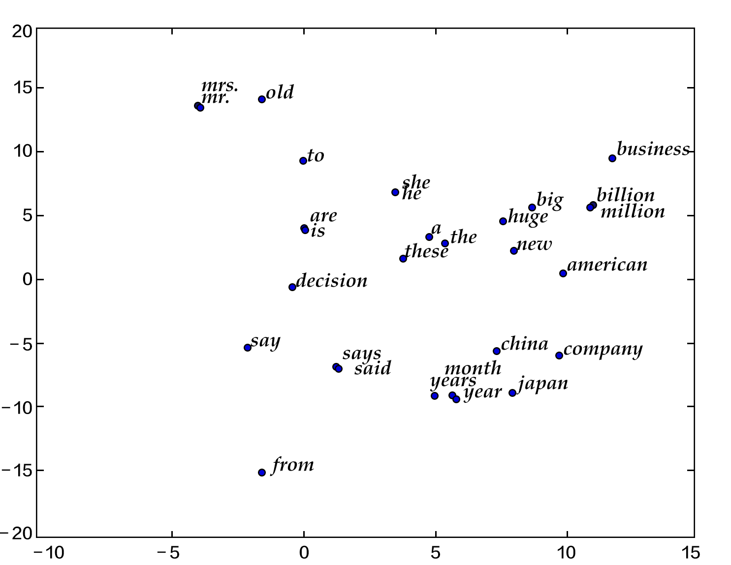## Results Demonstration In this section, we use the $t-$SNE\[[4](#reference)\] data visualization algorithm to draw the word embedding vectors after projecting them onto a two-dimensional space (see figure below). From the figure we can see that the semantically relevant words -- *a*, *the*, and *these* or *big* and *huge* -- are close to each other in the projected space, while irrelevant words -- *say* and *business* or *decision* and *japan* -- are far from each other.

Figure 1. Two dimension projection of word embeddings

### Cosine Similarity On the other hand, we know that the cosine similarity between two vectors falls between $[-1,1]$. Specifically, the cosine similarity is 1 when the vectors are identical, 0 when the vectors are perpendicular, -1 when the are of opposite directions. That is, the cosine similarity between two vectors scales with their relevance. So we can calculate the cosine similarity of two word embedding vectors to represent their relevance: ``` please input two words: big huge similarity: 0.899180685161 please input two words: from company similarity: -0.0997506977351 ``` The above results could be obtained by running `calculate_dis.py`, which loads the words in the dictionary and their corresponding trained word embeddings. For detailed instruction, see section [Model Application](https://github.com/PaddlePaddle/book/tree/develop/04.word2vec#model-application). ## Model Overview In this section, we will introduce three word embedding models: N-gram model, CBOW, and Skip-gram, which all output the frequency of each word given its immediate context. For N-gram model, we will first introduce the concept of language model, and implement it using PaddlePaddle in section [Training](https://github.com/PaddlePaddle/book/tree/develop/04.word2vec#model-application). The latter two models, which became popular recently, are neural word embedding model developed by Tomas Mikolov at Google \[[3](#reference)\]. Despite their apparent simplicity, these models train very well. ### Language Model Before diving into word embedding models, we will first introduce the concept of **language model**. Language models build the joint probability function $P(w_1, ..., w_T)$ of a sentence, where $w_i$ is the i-th word in the sentence. The goal is to give higher probabilities to meaningful sentences, and lower probabilities to meaningless constructions. In general, models that generate the probability of a sequence can be applied to many fields, like machine translation, speech recognition, information retrieval, part-of-speech tagging, and handwriting recognition. Take information retrieval, for example. If you were to search for "how long is a football bame" (where bame is a medical noun), the search engine would have asked if you had meant "how long is a football game" instead. This is because the probability of "how long is a football bame" is very low according to the language model; in addition, among all of the words easily confused with "bame", "game" would build the most probable sentence. #### Target Probability For language model's target probability $P(w_1, ..., w_T)$, if the words in the sentence were to be independent, the joint probability of the whole sentence would be the product of each word's probability: $$P(w_1, ..., w_T) = \prod_{t=1}^TP(w_t)$$ However, the frequency of words in a sentence typically relates to the words before them, so canonical language models are constructed using conditional probability in its target probability: $$P(w_1, ..., w_T) = \prod_{t=1}^TP(w_t | w_1, ... , w_{t-1})$$ ### N-gram neural model In computational linguistics, n-gram is an important method to represent text. An n-gram represents a contiguous sequence of n consecutive items given a text. Based on the desired application scenario, each item could be a letter, a syllable or a word. The N-gram model is also an important method in statistical language modeling. When training language models with n-grams, the first (n-1) words of an n-gram are used to predict the *n*th word. Yoshua Bengio and other scientists describe how to train a word embedding model using neural network in the famous paper of Neural Probabilistic Language Models \[[1](#reference)\] published in 2003. The Neural Network Language Model (NNLM) described in the paper learns the language model and word embedding simultaneously through a linear transformation and a non-linear hidden connection. That is, after training on large amounts of corpus, the model learns the word embedding; then, it computes the probability of the whole sentence, using the embedding. This type of language model can overcome the **curse of dimensionality** i.e. model inaccuracy caused by the difference in dimensionality between training and testing data. Note that the term *neural network language model* is ill-defined, so we will not use the name NNLM but only refer to it as *N-gram neural model* in this section. We have previously described language model using conditional probability, where the probability of the *t*-th word in a sentence depends on all $t-1$ words before it. Furthermore, since words further prior have less impact on a word, and every word within an n-gram is only effected by its previous n-1 words, we have: $$P(w_1, ..., w_T) = \prod_{t=n}^TP(w_t|w_{t-1}, w_{t-2}, ..., w_{t-n+1})$$ Given some real corpus in which all sentences are meaningful, the n-gram model should maximize the following objective function: $$\frac{1}{T}\sum_t f(w_t, w_{t-1}, ..., w_{t-n+1};\theta) + R(\theta)$$ where $f(w_t, w_{t-1}, ..., w_{t-n+1})$ represents the conditional logarithmic probability of the current word $w_t$ given its previous $n-1$ words, and $R(\theta)$ represents parameter regularization term.

Figure 2. N-gram neural network model

Figure 2 shows the N-gram neural network model. From the bottom up, the model has the following components: - For each sample, the model gets input $w_{t-n+1},...w_{t-1}$, and outputs the probability that the t-th word is one of `|V|` in the dictionary. Every input word $w_{t-n+1},...w_{t-1}$ first gets transformed into word embedding $C(w_{t-n+1}),...C(w_{t-1})$ through a transformation matrix. - All the word embeddings concatenate into a single vector, which is mapped (nonlinearly) into the $t$-th word hidden representation: $$g=Utanh(\theta^Tx + b_1) + Wx + b_2$$ where $x$ is the large vector concatenated from all the word embeddings representing the context; $\theta$, $U$, $b_1$, $b_2$ and $W$ are parameters connecting word embedding layers to the hidden layers. $g$ represents the unnormalized probability of the output word, $g_i$ represents the unnormalized probability of the output word being the i-th word in the dictionary. - Based on the definition of softmax, using normalized $g_i$, the probability that the output word is $w_t$ is represented as: $$P(w_t | w_1, ..., w_{t-n+1}) = \frac{e^{g_{w_t}}}{\sum_i^{|V|} e^{g_i}}$$ - The cost of the entire network is a multi-class cross-entropy and can be described by the following loss function $$J(\theta) = -\sum_{i=1}^N\sum_{c=1}^{|V|}y_k^{i}log(softmax(g_k^i))$$ where $y_k^i$ represents the true label for the $k$-th class in the $i$-th sample ($0$ or $1$), $softmax(g_k^i)$ represents the softmax probability for the $k$-th class in the $i$-th sample. 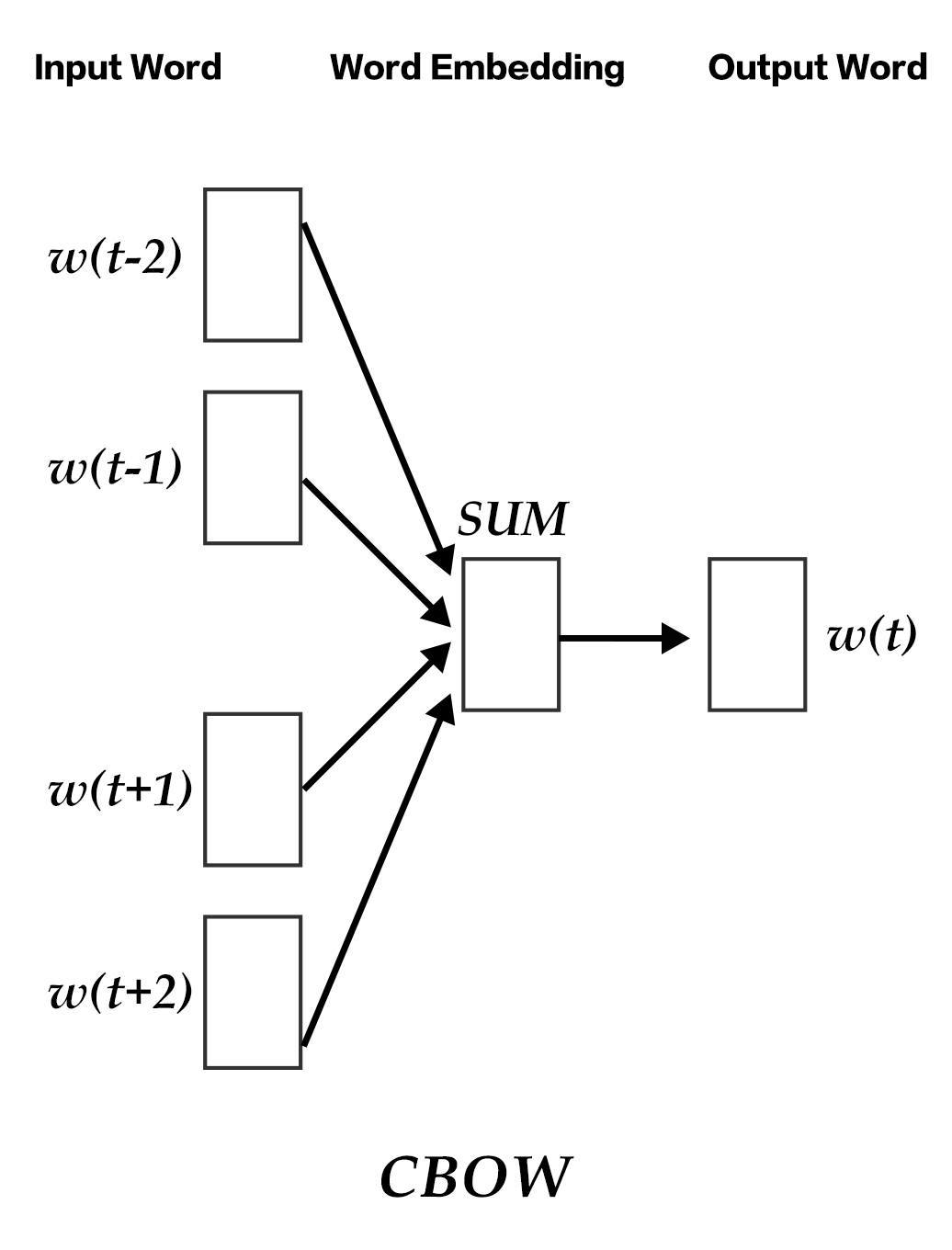### Continuous Bag-of-Words model(CBOW) CBOW model predicts the current word based on the N words both before and after it. When $N=2$, the model is as the figure below:

Figure 3. CBOW model

Specifically, by ignoring the order of words in the sequence, CBOW uses the average value of the word embedding of the context to predict the current word: $$\text{context} = \frac{x_{t-1} + x_{t-2} + x_{t+1} + x_{t+2}}{4}$$ where $x_t$ is the word embedding of the t-th word, classification score vector is $z=U*\text{context}$, the final classification $y$ uses softmax and the loss function uses multi-class cross-entropy. ### Skip-gram model The advantages of CBOW is that it smooths over the word embeddings of the context and reduces noise, so it is very effective on small dataset. Skip-gram uses a word to predict its context and get multiple context for the given word, so it can be used in larger datasets.

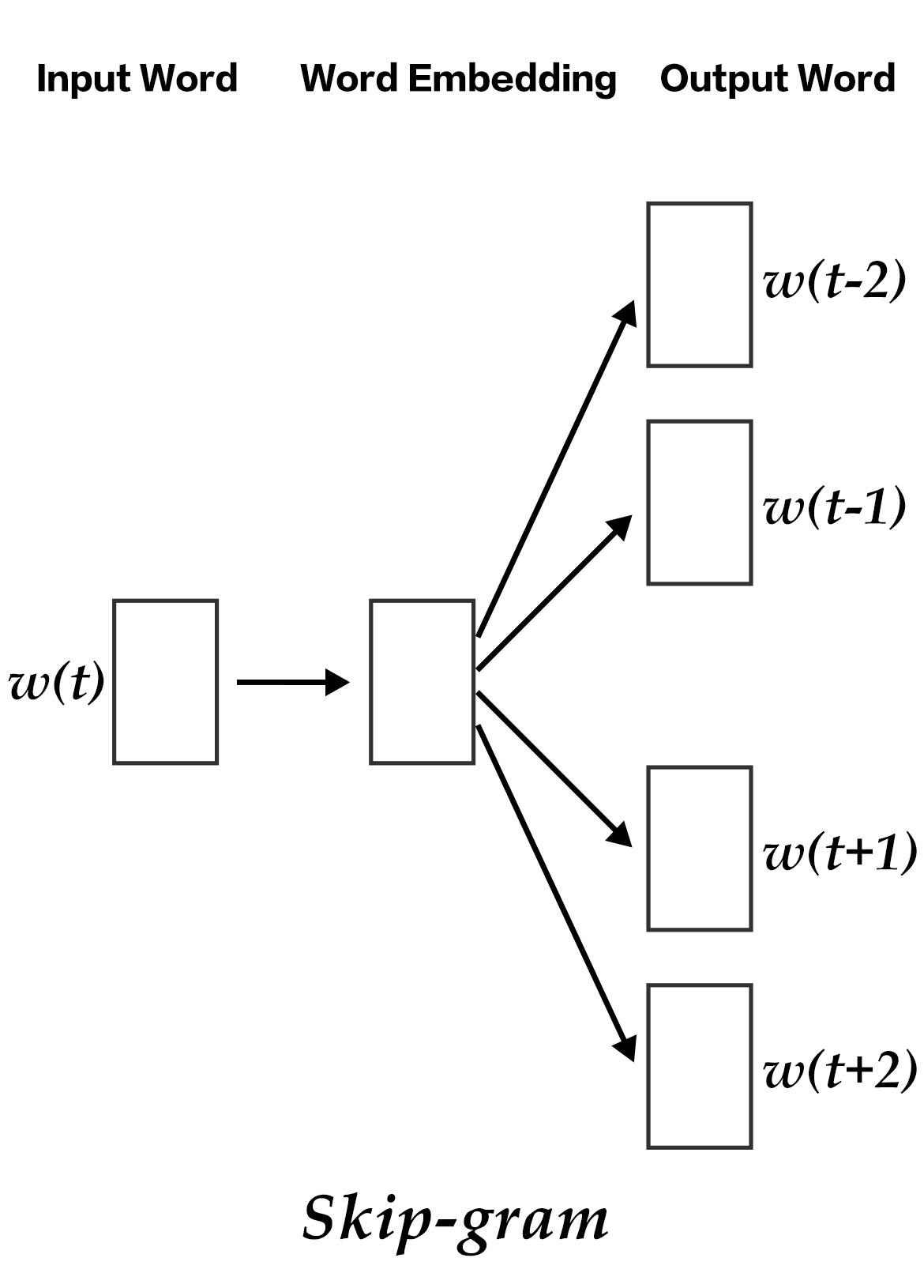
Figure 4. Skip-gram model

As illustrated in the figure above, skip-gram model maps the word embedding of the given word onto $2n$ word embeddings (including $n$ words before and $n$ words after the given word), and then combine the classification loss of all those $2n$ words by softmax. ## Dataset We will use Penn Treebank (PTB) (Tomas Mikolov's pre-processed version) dataset. PTB is a small dataset, used in Recurrent Neural Network Language Modeling Toolkit\[[2](#reference)\]. Its statistics are as follows:

training set	validation set	test set
ptb.train.txt	ptb.valid.txt	ptb.test.txt
42068 lines	3370 lines	3761 lines

### Python Dataset Module We encapsulated the PTB Data Set in our Python module `paddle.dataset.imikolov`. This module can 1. download the dataset to `~/.cache/paddle/dataset/imikolov`, if not yet, and 2. [preprocesses](#preprocessing) the dataset. ### Preprocessing We will be training a 5-gram model. Given five words in a window, we will predict the fifth word given the first four words. Beginning and end of a sentence have a special meaning, so we will add begin token `` in the front of the sentence. And end token `` in the end of the sentence. By moving the five word window in the sentence, data instances are generated. For example, the sentence "I have a dream that one day" generates five data instances: ```text I have a dream I have a dream that have a dream that one a dream that one day dream that one day ``` At last, each data instance will be converted into an integer sequence according it's words' index inside the dictionary. 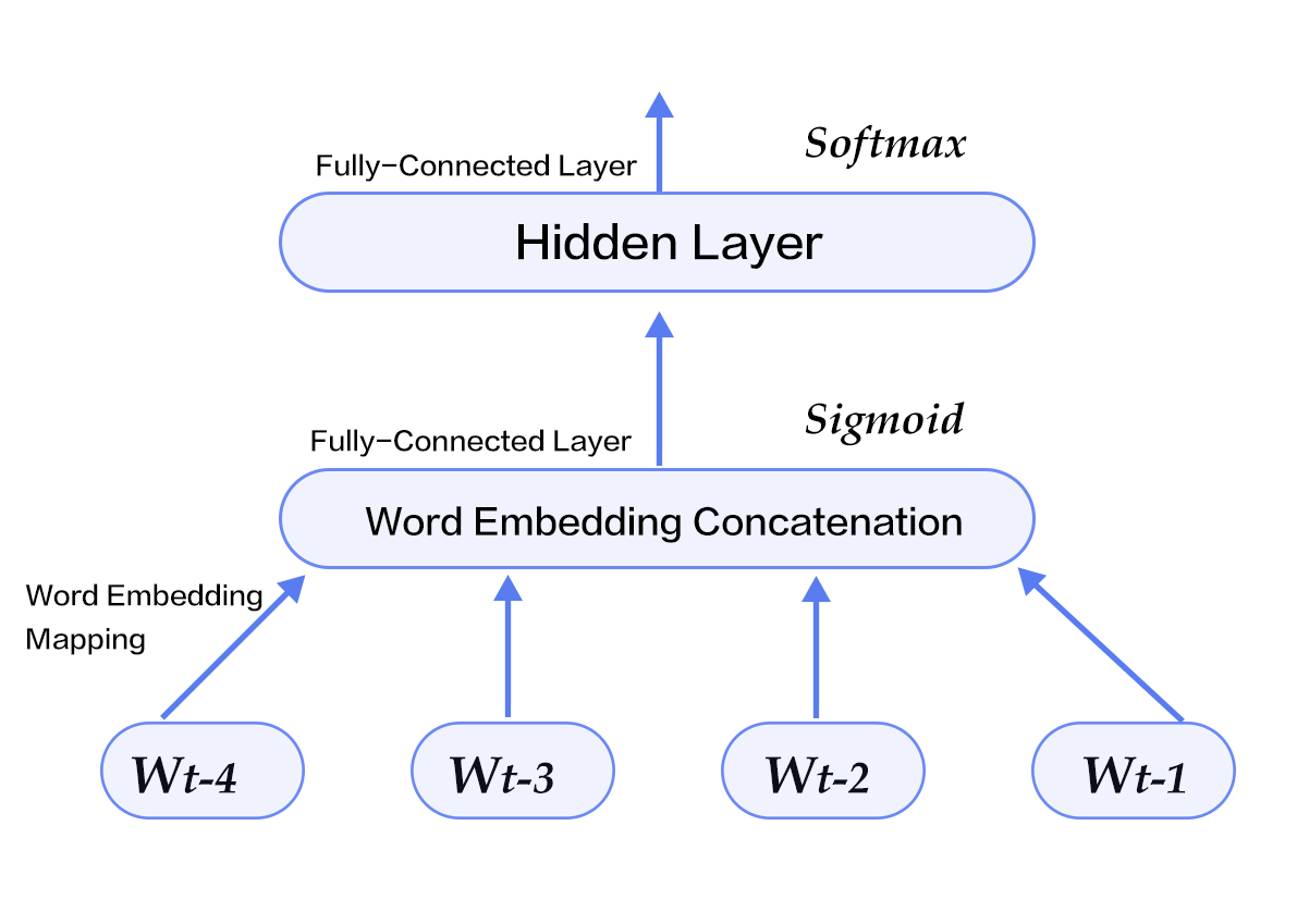## Training The neural network that we will be using is illustrated in the graph below:

Figure 5. N-gram neural network model in model configuration

`word2vec/train.py` demonstrates training word2vec using PaddlePaddle: - Import packages. ```python import math import paddle.v2 as paddle ``` - Configure parameter. ```python embsize = 32 # word vector dimension hiddensize = 256 # hidden layer dimension N = 5 # train 5-gram ``` - functions used to save and load word dict and embedding table ```python # save and load word dict and embedding table def save_dict_and_embedding(word_dict, embeddings): with open("word_dict", "w") as f: for key in word_dict: f.write(key + " " + str(word_dict[key]) + "\n") with open("embedding_table", "w") as f: numpy.savetxt(f, embeddings, delimiter=',', newline='\n') def load_dict_and_embedding(): word_dict = dict() with open("word_dict", "r") as f: for line in f: key, value = line.strip().split(" ") word_dict[key] = value embeddings = numpy.loadtxt("embedding_table", delimiter=",") return word_dict, embeddings ``` - Map the $n-1$ words $w_{t-n+1},...w_{t-1}$ before $w_t$ to a D-dimensional vector though matrix of dimention $|V|\times D$ (D=32 in this example). ```python def wordemb(inlayer): wordemb = paddle.layer.table_projection( input=inlayer, size=embsize, param_attr=paddle.attr.Param( name="_proj", initial_std=0.001, learning_rate=1, l2_rate=0, sparse_update=True)) return wordemb ``` - Define name and type for input to data layer. ```python paddle.init(use_gpu=False, trainer_count=3) word_dict = paddle.dataset.imikolov.build_dict() dict_size = len(word_dict) # Every layer takes integer value of range [0, dict_size) firstword = paddle.layer.data( name="firstw", type=paddle.data_type.integer_value(dict_size)) secondword = paddle.layer.data( name="secondw", type=paddle.data_type.integer_value(dict_size)) thirdword = paddle.layer.data( name="thirdw", type=paddle.data_type.integer_value(dict_size)) fourthword = paddle.layer.data( name="fourthw", type=paddle.data_type.integer_value(dict_size)) nextword = paddle.layer.data( name="fifthw", type=paddle.data_type.integer_value(dict_size)) Efirst = wordemb(firstword) Esecond = wordemb(secondword) Ethird = wordemb(thirdword) Efourth = wordemb(fourthword) ``` - Concatenate n-1 word embedding vectors into a single feature vector. ```python contextemb = paddle.layer.concat(input=[Efirst, Esecond, Ethird, Efourth]) ``` - Feature vector will go through a fully connected layer which outputs a hidden feature vector. ```python hidden1 = paddle.layer.fc(input=contextemb, size=hiddensize, act=paddle.activation.Sigmoid(), layer_attr=paddle.attr.Extra(drop_rate=0.5), bias_attr=paddle.attr.Param(learning_rate=2), param_attr=paddle.attr.Param( initial_std=1. / math.sqrt(embsize * 8), learning_rate=1)) ``` - Hidden feature vector will go through another fully conected layer, turn into a $|V|$ dimensional vector. At the same time softmax will be applied to get the probability of each word being generated. ```python predictword = paddle.layer.fc(input=hidden1, size=dict_size, bias_attr=paddle.attr.Param(learning_rate=2), act=paddle.activation.Softmax()) ``` - We will use cross-entropy cost function. ```python cost = paddle.layer.classification_cost(input=predictword, label=nextword) ``` - Create parameter, optimizer and trainer. ```python parameters = paddle.parameters.create(cost) adagrad = paddle.optimizer.AdaGrad( learning_rate=3e-3, regularization=paddle.optimizer.L2Regularization(8e-4)) trainer = paddle.trainer.SGD(cost, parameters, adagrad) ``` Next, we will begin the training process. `paddle.dataset.imikolov.train()` and `paddle.dataset.imikolov.test()` is our training set and test set. Both of the function will return a **reader**: In PaddlePaddle, reader is a python function which returns a Python iterator which output a single data instance at a time. `paddle.batch` takes reader as input, outputs a **batched reader**: In PaddlePaddle, a reader outputs a single data instance at a time but batched reader outputs a minibatch of data instances. ```python def event_handler(event): if isinstance(event, paddle.event.EndIteration): if event.batch_id % 100 == 0: print "Pass %d, Batch %d, Cost %f, %s" % ( event.pass_id, event.batch_id, event.cost, event.metrics) if isinstance(event, paddle.event.EndPass): result = trainer.test( paddle.batch( paddle.dataset.imikolov.test(word_dict, N), 32)) print "Pass %d, Testing metrics %s" % (event.pass_id, result.metrics) with open("model_%d.tar"%event.pass_id, 'w') as f: parameters.to_tar(f) trainer.train( paddle.batch(paddle.dataset.imikolov.train(word_dict, N), 32), num_passes=100, event_handler=event_handler) ``` `trainer.train` will start training, the output of `event_handler` will be similar to following: ```text Pass 0, Batch 0, Cost 7.870579, {'classification_error_evaluator': 1.0}, Testing metrics {'classification_error_evaluator': 0.999591588973999} Pass 0, Batch 100, Cost 6.136420, {'classification_error_evaluator': 0.84375}, Testing metrics {'classification_error_evaluator': 0.8328699469566345} Pass 0, Batch 200, Cost 5.786797, {'classification_error_evaluator': 0.8125}, Testing metrics {'classification_error_evaluator': 0.8328542709350586} ... ``` After 30 passes, we can get average error rate around 0.735611. ## Save word dict and embedding table after training, we can save the word dict and embedding table for the future usage. ```python # save word dict and embedding table embeddings = parameters.get("_proj").reshape(len(word_dict), embsize) save_dict_and_embedding(word_dict, embeddings) ``` ## Model Application After the model is trained, we can load the saved model parameters and use it for other models. We can also use the parameters in various applications. ### Viewing Word Vector Parameters trained by PaddlePaddle can be viewed by `parameters.get()`. For example, we can check the word vector for word `apple`. ```python embeddings = parameters.get("_proj").reshape(len(word_dict), embsize) print embeddings[word_dict['apple']] ``` ```text [-0.38961065 -0.02392169 -0.00093231 0.36301503 0.13538605 0.16076435 -0.0678709 0.1090285 0.42014077 -0.24119169 -0.31847557 0.20410083 0.04910378 0.19021918 -0.0122014 -0.04099389 -0.16924137 0.1911236 -0.10917275 0.13068172 -0.23079982 0.42699069 -0.27679482 -0.01472992 0.2069038 0.09005053 -0.3282454 0.12717034 -0.24218646 0.25304323 0.19072419 -0.24286366] ``` ### Modifying Word Vector Word vectors (`embeddings`) that we get is a numpy array. We can modify this array and set it back to `parameters`. ```python def modify_embedding(emb): # Add your modification here. pass modify_embedding(embeddings) parameters.set("_proj", embeddings) ``` ### Calculating Cosine Similarity Cosine similarity is one way of quantifying the similarity between two vectors. The range of result is $[-1, 1]$. The bigger the value, the similar two vectors are: ```python from scipy import spatial emb_1 = embeddings[word_dict['world']] emb_2 = embeddings[word_dict['would']] print spatial.distance.cosine(emb_1, emb_2) ``` ```text 0.99375076448 ``` ## Conclusion This chapter introduces word embeddings, the relationship between language model and word embedding, and how to train neural networks to learn word embedding. In information retrieval, the relevance between the query and document keyword can be computed through the cosine similarity of their word embeddings. In grammar analysis and semantic analysis, a previously trained word embedding can initialize models for better performance. In document classification, clustering the word embedding can group synonyms in the documents. We hope that readers can use word embedding models in their work after reading this chapter. ## Referenes 1. Bengio Y, Ducharme R, Vincent P, et al. [A neural probabilistic language model](http://www.jmlr.org/papers/volume3/bengio03a/bengio03a.pdf)[J]. journal of machine learning research, 2003, 3(Feb): 1137-1155. 2. Mikolov T, Kombrink S, Deoras A, et al. [Rnnlm-recurrent neural network language modeling toolkit](http://www.fit.vutbr.cz/~imikolov/rnnlm/rnnlm-demo.pdf)[C]//Proc. of the 2011 ASRU Workshop. 2011: 196-201. 3. Mikolov T, Chen K, Corrado G, et al. [Efficient estimation of word representations in vector space](https://arxiv.org/pdf/1301.3781.pdf)[J]. arXiv preprint arXiv:1301.3781, 2013. 4. Maaten L, Hinton G. [Visualizing data using t-SNE](https://lvdmaaten.github.io/publications/papers/JMLR_2008.pdf)[J]. Journal of Machine Learning Research, 2008, 9(Nov): 2579-2605. 5. https://en.wikipedia.org/wiki/Singular_value_decomposition
This tutorial is contributed by PaddlePaddle, and licensed under a Creative Commons Attribution-ShareAlike 4.0 International License.