# Semantic Role Labeling
Source code of this chapter is in [book/label_semantic_roles](https://github.com/PaddlePaddle/book/tree/develop/label_semantic_roles).
## Background
Natural Language Analysis contains three components: Lexical Analysis, Syntactic Analysis, and Semantic Analysis. Semantic Role Labelling (SRL) is one way for Shallow Semantic Analysis. A predicate of a sentence is a property that a subject possesses or is characterized, such as what it does, what it is or how it is, which mostly corresponds to the core of an event. The noun associated with a predicate is called Argument. Semantic roles express the abstract roles that arguments of a predicate can take in the event, such as Agent, Patient, Theme, Experiencer, Beneficiary, Instrument, Location, Goal and Source, etc.
In the following example, “遇到” (encounters) is a Predicate (“Pred”),“小明” (Ming) is an Agent,“小红” (Hong) is a Patient,“昨天” (yesterday) indicates the Time, and “公园” (park) is the Location.
$$\mbox{[小明]}_{\mbox{Agent}}\mbox{[昨天]}_{\mbox{Time}}\mbox{[晚上]}_\mbox{Time}\mbox{在[公园]}_{\mbox{Location}}\mbox{[遇到]}_{\mbox{Predicate}}\mbox{了[小红]}_{\mbox{Patient}}\mbox{。}$$
Instead of in-depth analysis on semantic information, the goal of Semantic Role Labeling is to identify the relation of predicate and other constituents, e.g., predicate-argument structure, as specific semantic roles, which is an important intermediate step in a wide range of natural language understanding tasks (Information Extraction, Discourse Analysis, DeepQA etc). Predicates are always assumed to be given; the only thing is to identify arguments and their semantic roles.
Standard SRL system mostly builds on top of Syntactic Analysis and contains five steps:
1. Construct a syntactic parse tree, as shown in Fig. 1
2. Identity candidate arguments of given predicate from constructed syntactic parse tree.
3. Prune most unlikely candidate arguments.
4. Identify arguments, often by a binary classifier.
5. Multi-class semantic role labeling. Steps 2-3 usually introduce hand-designed features based on Syntactic Analysis (step 1).

Fig 1. Syntactic parse tree
核心关系-> HED
定中关系-> ATT
主谓关系-> SBV
状中结构-> ADV
介宾关系-> POB
右附加关系-> RAD
动宾关系-> VOB
标点-> WP
However, complete syntactic analysis requires identifying the relation among all constitutes and the performance of SRL is sensitive to the precision of syntactic analysis, which makes SRL a very challenging task. To reduce the complexity and obtain some syntactic structure information, we often use shallow syntactic analysis. Shallow Syntactic Analysis is also called partial parsing or chunking. Unlike complete syntactic analysis which requires the construction of the complete parsing tree, Shallow Syntactic Analysis only need to identify some independent components with relatively simple structure, such as verb phrases (chunk). To avoid difficulties in constructing a syntactic tree with high accuracy, some work\[[1](#Reference)\] proposed semantic chunking based SRL methods, which convert SRL as a sequence tagging problem. Sequence tagging tasks classify syntactic chunks using BIO representation. For syntactic chunks forming a chunk of type A, the first chunk receives the B-A tag (Begin), the remaining ones receive the tag I-A (Inside), and all chunks outside receive the tag O-A.
The BIO representation of above example is shown in Fig.1.
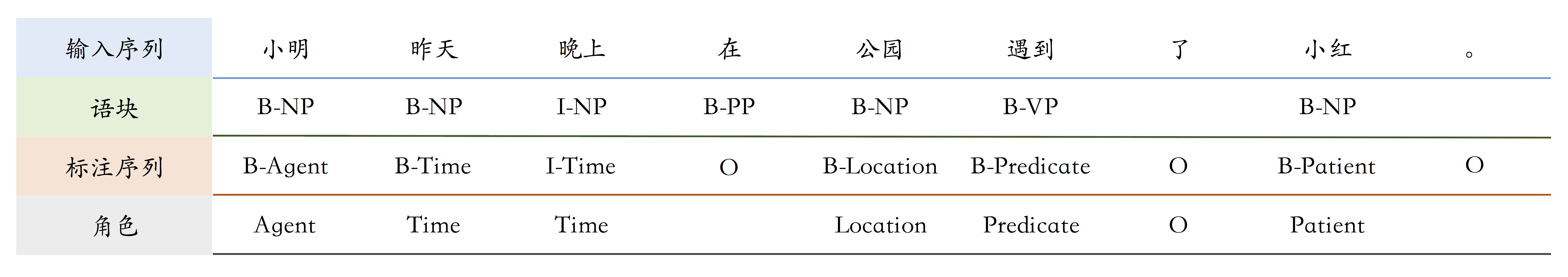
Fig 2. BIO represention
输入序列-> input sequence
语块-> chunk
标注序列-> label sequence
角色-> role
This example illustrates the simplicity of sequence tagging because (1) shallow syntactic analysis reduces the precision requirement of syntactic analysis; (2) pruning candidate arguments is removed; 3) argument identification and tagging are finished at the same time. Such unified methods simplify the procedure, reduce the risk of accumulating errors and boost the performance further.
In this tutorial, our SRL system is built as an end-to-end system via a neural network. We take only text sequences, without using any syntactic parsing results or complex hand-designed features. We give public dataset [CoNLL-2004 and CoNLL-2005 Shared Tasks](http://www.cs.upc.edu/~srlconll/) as an example to illustrate: given a sentence with predicates marked, identify the corresponding arguments and their semantic roles by sequence tagging method.
## Model
Recurrent Neural Networks are important tools for sequence modeling and have been successfully used in some natural language processing tasks. Unlike Feed-forward neural networks, RNNs can model the dependency between elements of sequences. LSTMs as variants of RNNs aim to model long-term dependency in long sequences. We have introduced this in [understand_sentiment](https://github.com/PaddlePaddle/book/tree/develop/understand_sentiment). In this chapter, we continue to use LSTMs to solve SRL problems.
### Stacked Recurrent Neural Network
Deep Neural Networks allows extracting hierarchical representations. Higher layers can form more abstract/complex representations on top of lower layers. LSTMs, when unfolded in time, is a deep feed-forward neural network, because a computational path between the input at time $k < t$ to the output at time $t$ crosses several nonlinear layers. However, the computation carried out at each time-step is only linear transformation, which makes LSTMs a shallow model. Deep LSTMs are typically constructed by stacking multiple LSTM layers on top of each other and taking the output from lower LSTM layer at time $t$ as the input of upper LSTM layer at time $t$. Deep, hierarchical neural networks can be much efficient at representing some functions and modeling varying-length dependencies\[[2](#Reference)\].
However, deep LSTMs increases the number of nonlinear steps the gradient has to traverse when propagated back in depth. For example, four layer LSTMs can be trained properly, but the performance becomes worse as the number of layers up to 4-8. Conventional LSTMs prevent backpropagated errors from vanishing and exploding by introducing shortcut connections to skip the intermediate nonlinear layers. Therefore, deep LSTMs can consider shortcut connections in depth as well.
The operation of a single LSTM cell contain 3 parts: (1) input-to-hidden: map input $x$ to the input of the forget gates, input gates, memory cells and output gates by linear transformation (i.e., matrix mapping); (2) hidden-to-hidden: calculate forget gates, input gates, output gates and update memory cell, this is the main part of LSTMs; (3)hidden-to-output: this part typically involves an activation operation on hidden states. Based on the stacked LSTMs, we add a shortcut connection: take the input-to-hidden from the previous layer as a new input and learn another linear transformation.
Fig.3 illustrate the final stacked recurrent neural networks.
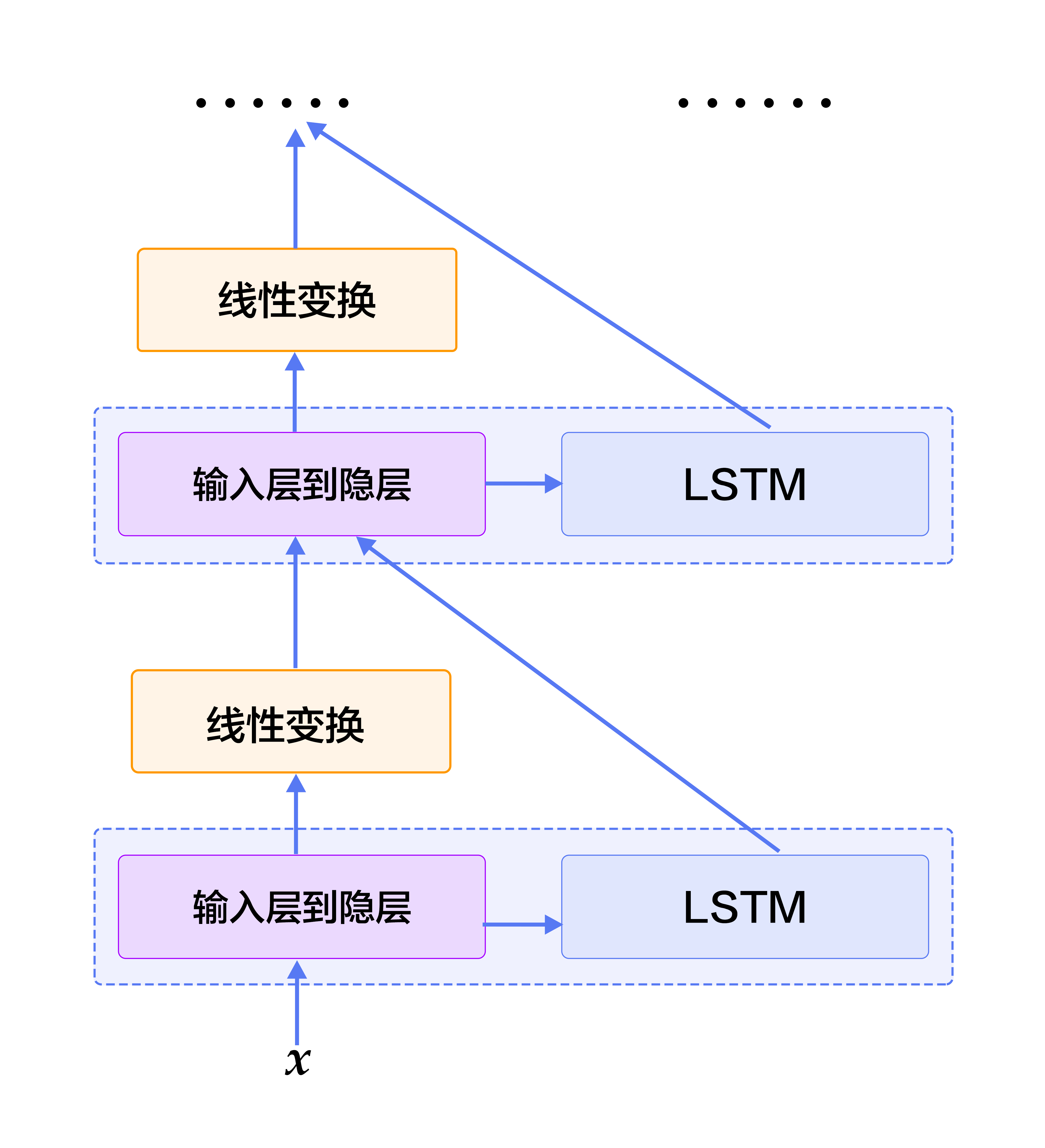
Fig 3. Stacked Recurrent Neural Networks
线性变换-> linear transformation
输入层到隐层-> input-to-hidden
### Bidirectional Recurrent Neural Network
LSTMs can summarize the history of previous inputs seen up to now, but can not see the future. In most of NLP (natural language processing) tasks, the entire sentences are ready to use. Therefore, sequential learning might be much efficient if the future can be encoded as well like histories.
To address the above drawbacks, we can design bidirectional recurrent neural networks by making a minor modification. Higher LSTM layers process the sequence in reversed direction with previous lower LSTM layers, i.e., Deep LSTMs operate from left-to-right, right-to-left, left-to-right,..., in depth. Therefore, LSTM layers at time-step $t$ can see both histories and the future since the second layer. Fig. 4 illustrates the bidirectional recurrent neural networks.
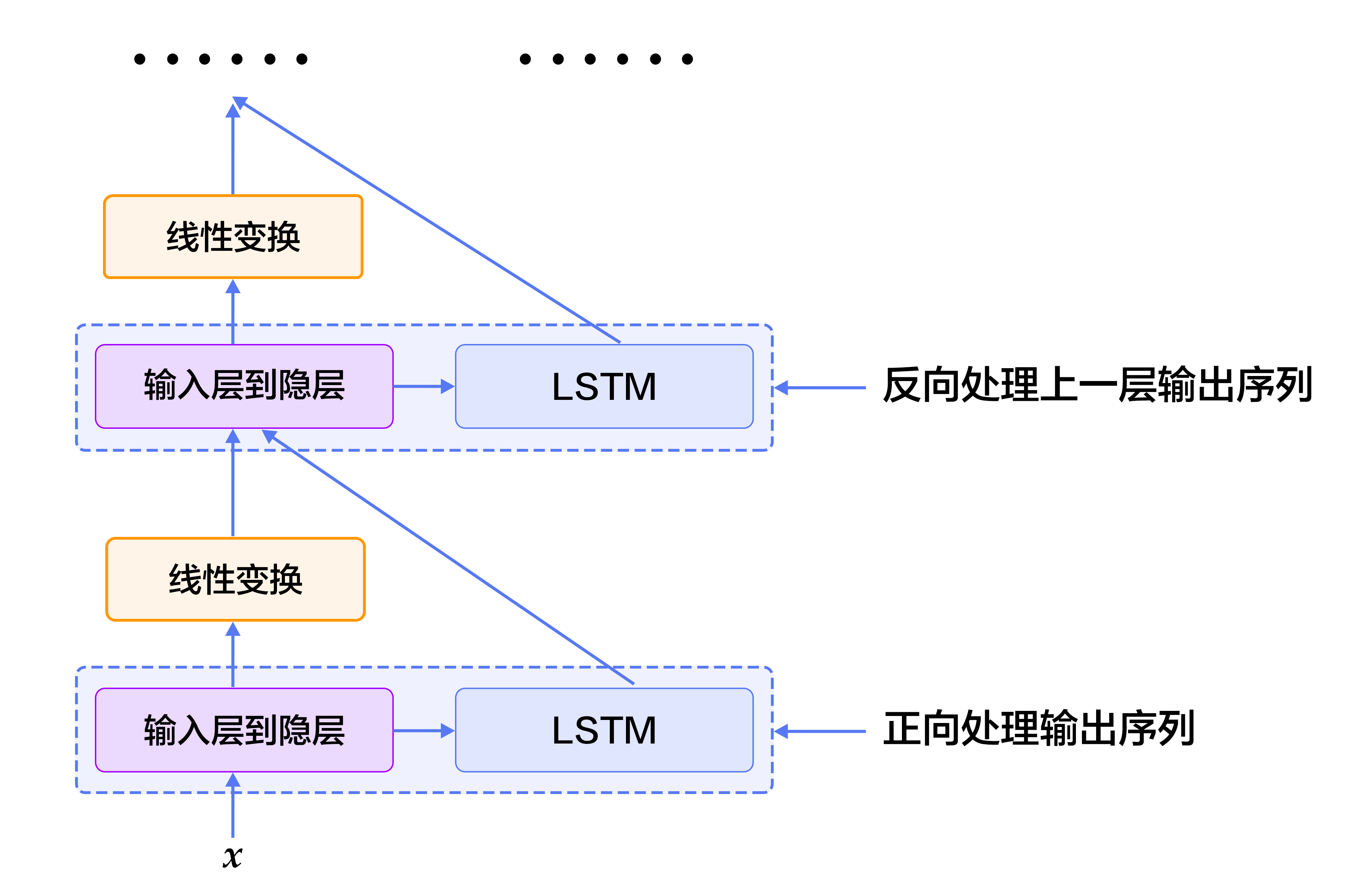
Fig 4. Bidirectional LSTMs
线性变换-> linear transformation
输入层到隐层-> input-to-hidden
正向处理输出序列->process sequence in the forward direction
反向处理上一层序列-> process sequence from the previous layer in backward direction
Note that, this bidirectional RNNs is different with the one proposed by Bengio et al. in machine translation tasks \[[3](#Reference), [4](#Reference)\]. We will introduce another bidirectional RNNs in the following tasks[machine translation](https://github.com/PaddlePaddle/book/blob/develop/machine_translation/README.md)
### Conditional Random Field
The basic pipeline of Neural Networks solving problems is 1) all lower layers aim to learn representations; 2) the top layer is designed for learning the final task. In SRL tasks, CRF is built on top of the network for the final tag sequence prediction. It takes the representations provided by the last LSTM layer as input.
CRF is a probabilistic graph model (undirected) with nodes denoting random variables and edges denoting dependencies between nodes. To be simplicity, CRFs learn conditional probability $P(Y|X)$, where $X = (x_1, x_2, ... , x_n)$ are sequences of input, $Y = (y_1, y_2, ... , y_n)$ are label sequences; Decoding is to search sequence $Y$ to maximize conditional probability $P(Y|X)$, i.e., $Y^* = \mbox{arg max}_{Y} P(Y | X)$。
Sequence tagging tasks only consider input and output as linear sequences without extra dependent assumptions on graph model. Thus, the graph model of sequence tagging tasks is simple chain or line, which results in a Linear-Chain Conditional Random Field, shown in Fig.5.

Fig 5. Linear Chain Conditional Random Field used in SRL tasks
By the fundamental theorem of random fields \[[5](#Reference)\], the joint distribution over the label sequence $Y$ given $X$ has the form:
$$p(Y | X) = \frac{1}{Z(X)} \text{exp}\left(\sum_{i=1}^{n}\left(\sum_{j}\lambda_{j}t_{j} (y_{i - 1}, y_{i}, X, i) + \sum_{k} \mu_k s_k (y_i, X, i)\right)\right)$$
where, $Z(X)$ is normalization constant, $t_j$ is feature function defined on edges, called transition feature, depending on $y_i$ and $y_{i-1}$ which represents transition probabilities from $y_{i-1}$ to $y_i$ given input sequence $X$. $s_k$ is feature function defined on nodes, called state feature, depending on $y_i$ and represents the probality of $y_i$ given input sequence $X$. $\lambda_j$ 和 $\mu_k$ are weights corresponding to $t_j$ and $s_k$. Actually, $t$ and $s$ can be wrtten in the same form, then take summation over all nodes $i$: $f_{k}(Y, X) = \sum_{i=1}^{n}f_k({y_{i - 1}, y_i, X, i})$, $f$ is defined as feature function. Thus, $P(Y|X)$ can be wrtten as:
$$p(Y|X, W) = \frac{1}{Z(X)}\text{exp}\sum_{k}\omega_{k}f_{k}(Y, X)$$
$\omega$ are weights of feature function which should be learned in CRF models. At training stage, given input sequences and label sequences $D = \left[(X_1, Y_1), (X_2 , Y_2) , ... , (X_N, Y_N)\right]$, solve following objective function using MLE:
$$L(\lambda, D) = - \text{log}\left(\prod_{m=1}^{N}p(Y_m|X_m, W)\right) + C \frac{1}{2}\lVert W\rVert^{2}$$
This objective function can be solved via back-propagation in an end-to-end manner. At decoding stage, given input sequences $X$, search sequence $\bar{Y}$ to maximize conditional probability $\bar{P}(Y|X)$ via decoding methods (such as Viterbi, Beam Search).
### DB-LSTM SRL model
Given predicates and a sentence, SRL tasks aim to identify arguments of the given predicate and their semantic roles. If a sequence has n predicates, we will process this sequence n times. One model is as follows:
1. Construct inputs;
- input 1: predicate, input 2: sentence
- expand input 1 as a sequence with the same length with input 2 using one-hot representation;
2. Convert one-hot sequences from step 1 to vector sequences via lookup table;
3. Learn the representation of input sequences by taking vector sequences from step 2 as inputs;
4. Take representations from step 3 as inputs, label sequence as supervision signal, do sequence tagging tasks
We can try above method. Here, we propose some modifications by introducing two simple but effective features:
- predicate context (ctx-p): A single predicate word can not exactly describe the predicate information, especially when the same words appear more than one times in a sentence. With the expanded context, the ambiguity can be largely eliminated. Thus, we extract $n$ words before and after predicate to construct a window chunk.
- region mark ($m_r$): $m_r = 1$ to denote word in that position locates in the predicate context region, or $m_r = 0$ if not.
After modification, the model is as follows:
1. Construct inputs
- Input 1: word sequence. Input 2: predicate. Input 3: predicate context, extract $n$ words before and after predicate. Input 4: region mark sequence, element value will be 1 if word locates in the predicate context region, 0 otherwise.
- expand input 2~3 as sequences with the same length with input 1
2. Convert input 1~4 to vector sequences via lookup table; input 1 and 3 shares the same lookup table, input 2 and 4 have separate lookup tables
3. Take four vector sequences from step 2 as inputs of bidirectional LSTMs; Train LSTMs to update representations
4. Take representation from step 3 as input of CRF, label sequence as supervision signal, do sequence tagging tasks

Fig 6. DB-LSTM for SRL tasks
论元-> argu
谓词-> pred
谓词上下文-> ctx-p
谓词上下文区域标记-> $m_r$
输入-> input
原句-> sentence
反向LSTM-> LSTM Reverse
## Data Preparation
In the tutorial, we use [CoNLL 2005](http://www.cs.upc.edu/~srlconll/) SRL task open dataset as an example. It is important to note that the training set and development set of the CoNLL 2005 SRL task are not free to download after the competition. Currently, only the test set can be obtained, including 23 sections of the Wall Street Journal and three sections of the Brown corpus. In this tutorial, we use the WSJ corpus as the training dataset to explain the model. However, since the training set is small, if you want to train a usable neural network SRL system, consider paying for the full corpus.
The original data includes a variety of information such as POS tagging, naming entity recognition, parsing tree, and so on. In this tutorial, we only use the data under the words folder (text sequence) and the props folder (label results) inside test.wsj parent folder. The data directory used in this tutorial is as follows:
```text
conll05st-release/
└── test.wsj
├── props # 标注结果
└── words # 输入文本序列
```
The annotation information is derived from the results of Penn TreeBank\[[7](#references)\] and PropBank \[[8](# references)\]. The label of the PropBank is different from the label that we used in the example at the beginning of the article, but the principle is the same. For the description of the label, please refer to the paper \[[9](#references)\].
The raw data needs to be preprocessed before used by PaddlePaddle. The preprocessing consists of the following steps:
1. Merge the text sequence and the tag sequence into the same record;
2. If a sentence contains $n$ predicates, the sentence will be processed $n$ times into $n$ separate training samples, each sample with a different predicate;
3. Extract the predicate context and construct the predicate context region marker;
4. Construct the markings in BIO format;
5. Obtain the integer index corresponding to the word according to the dictionary.
```python
# import paddle.v2.dataset.conll05 as conll05
# conll05.corpus_reader does step 1 and 2 as mentioned above.
# conll05.reader_creator does step 3 to 5.
# conll05.test gets preprocessed training instances.
```
After preprocessing completes, a training sample contains nine features, namely: word sequence, predicate, predicate context (5 columns), region mark sequence, label sequence. Following table is an example of a training sample.
| word sequence | predicate | predicate context(5 columns) | region mark sequence | label sequence|
|---|---|---|---|---|
| A | set | n't been set . × | 0 | B-A1 |
| record | set | n't been set . × | 0 | I-A1 |
| date | set | n't been set . × | 0 | I-A1 |
| has | set | n't been set . × | 0 | O |
| n't | set | n't been set . × | 1 | B-AM-NEG |
| been | set | n't been set . × | 1 | O |
| set | set | n't been set . × | 1 | B-V |
| . | set | n't been set . × | 1 | O |
In addition to the data, we provide following resources:
| filename | explanation |
|---|---|
| word_dict | dictionary of input sentences, total 44068 words |
| label_dict | dictionary of labels, total 106 labels |
| predicate_dict | predicate dictionary, total 3162 predicates |
| emb | a pre-trained word vector lookup table, 32-dimentional |
We trained in the English Wikipedia language model to get a word vector lookup table used to initialize the SRL model. During the SRL model training process, the word vector lookup table is no longer updated. About the language model and the word vector lookup table can refer to [word vector](https://github.com/PaddlePaddle/book/blob/develop/word2vec/README.md) tutorial. There are 995,000,000 token in training corpus, and the dictionary size is 4900,000 words. In the CoNLL 2005 training corpus, 5% of the words are not in the 4900,000 words, and we see them all as unknown words, represented by ``.
Get dictionary, print dictionary size:
```python
import math
import numpy as np
import paddle.v2 as paddle
import paddle.v2.dataset.conll05 as conll05
word_dict, verb_dict, label_dict = conll05.get_dict()
word_dict_len = len(word_dict)
label_dict_len = len(label_dict)
pred_len = len(verb_dict)
print word_dict_len
print label_dict_len
print pred_len
```
## Model configuration
- 1. Define input data dimensions and model hyperparameters.
```python
mark_dict_len = 2 # Value range of region mark. Region mark is either 0 or 1, so range is 2
word_dim = 32 # word vector dimension
mark_dim = 5 # adjacent dimension
hidden_dim = 512 # the dimension of LSTM hidden layer vector is 128 (512/4)
depth = 8 # depth of stacked LSTM
# There are 9 features per sample, so we will define 9 data layers.
# They type for each layer is integer_value_sequence.
def d_type(value_range):
return paddle.data_type.integer_value_sequence(value_range)
# word sequence
word = paddle.layer.data(name='word_data', type=d_type(word_dict_len))
# predicate
predicate = paddle.layer.data(name='verb_data', type=d_type(pred_len))
# 5 features for predicate context
ctx_n2 = paddle.layer.data(name='ctx_n2_data', type=d_type(word_dict_len))
ctx_n1 = paddle.layer.data(name='ctx_n1_data', type=d_type(word_dict_len))
ctx_0 = paddle.layer.data(name='ctx_0_data', type=d_type(word_dict_len))
ctx_p1 = paddle.layer.data(name='ctx_p1_data', type=d_type(word_dict_len))
ctx_p2 = paddle.layer.data(name='ctx_p2_data', type=d_type(word_dict_len))
# region marker sequence
mark = paddle.layer.data(name='mark_data', type=d_type(mark_dict_len))
# label sequence
target = paddle.layer.data(name='target', type=d_type(label_dict_len))
```
Speciala note: hidden_dim = 512 means LSTM hidden vector of 128 dimension (512/4). Please refer PaddlePaddle official documentation for detail: [lstmemory](http://www.paddlepaddle.org/doc/ui/api/trainer_config_helpers/layers.html#lstmemory)。
- 2. The word sequence, predicate, predicate context, and region mark sequence are transformed into embedding vector sequences.
```python
# Since word vectorlookup table is pre-trained, we won't update it this time.
# is_static being True prevents updating the lookup table during training.
emb_para = paddle.attr.Param(name='emb', initial_std=0., is_static=True)
# hyperparameter configurations
default_std = 1 / math.sqrt(hidden_dim) / 3.0
std_default = paddle.attr.Param(initial_std=default_std)
std_0 = paddle.attr.Param(initial_std=0.)
predicate_embedding = paddle.layer.embedding(
size=word_dim,
input=predicate,
param_attr=paddle.attr.Param(
name='vemb', initial_std=default_std))
mark_embedding = paddle.layer.embedding(
size=mark_dim, input=mark, param_attr=std_0)
word_input = [word, ctx_n2, ctx_n1, ctx_0, ctx_p1, ctx_p2]
emb_layers = [
paddle.layer.embedding(
size=word_dim, input=x, param_attr=emb_para) for x in word_input
]
emb_layers.append(predicate_embedding)
emb_layers.append(mark_embedding)
```
- 3. 8 LSTM units will be trained in "forward / backward" order.
```python
hidden_0 = paddle.layer.mixed(
size=hidden_dim,
bias_attr=std_default,
input=[
paddle.layer.full_matrix_projection(
input=emb, param_attr=std_default) for emb in emb_layers
])
mix_hidden_lr = 1e-3
lstm_para_attr = paddle.attr.Param(initial_std=0.0, learning_rate=1.0)
hidden_para_attr = paddle.attr.Param(
initial_std=default_std, learning_rate=mix_hidden_lr)
lstm_0 = paddle.layer.lstmemory(
input=hidden_0,
act=paddle.activation.Relu(),
gate_act=paddle.activation.Sigmoid(),
state_act=paddle.activation.Sigmoid(),
bias_attr=std_0,
param_attr=lstm_para_attr)
# stack L-LSTM and R-LSTM with direct edges
input_tmp = [hidden_0, lstm_0]
for i in range(1, depth):
mix_hidden = paddle.layer.mixed(
size=hidden_dim,
bias_attr=std_default,
input=[
paddle.layer.full_matrix_projection(
input=input_tmp[0], param_attr=hidden_para_attr),
paddle.layer.full_matrix_projection(
input=input_tmp[1], param_attr=lstm_para_attr)
])
lstm = paddle.layer.lstmemory(
input=mix_hidden,
act=paddle.activation.Relu(),
gate_act=paddle.activation.Sigmoid(),
state_act=paddle.activation.Sigmoid(),
reverse=((i % 2) == 1),
bias_attr=std_0,
param_attr=lstm_para_attr)
input_tmp = [mix_hidden, lstm]
```
- 4. We will concatenate the output of top LSTM unit with it's input, and project into a hidden layer. Then put a fully connected layer on top of it to get the final vector representation.
```python
feature_out = paddle.layer.mixed(
size=label_dict_len,
bias_attr=std_default,
input=[
paddle.layer.full_matrix_projection(
input=input_tmp[0], param_attr=hidden_para_attr),
paddle.layer.full_matrix_projection(
input=input_tmp[1], param_attr=lstm_para_attr)
], )
```
- 5. We use CRF as cost function, the parameter of CRF cost will be named `crfw`.
```python
crf_cost = paddle.layer.crf(
size=label_dict_len,
input=feature_out,
label=target,
param_attr=paddle.attr.Param(
name='crfw',
initial_std=default_std,
learning_rate=mix_hidden_lr))
```
- 6. CRF decoding layer is used for evaluation and inference. It shares parameter with CRF layer. The sharing of parameters among multiple layers is specified by the same parameter name in these layers.
```python
crf_dec = paddle.layer.crf_decoding(
name='crf_dec_l',
size=label_dict_len,
input=feature_out,
label=target,
param_attr=paddle.attr.Param(name='crfw'))
```
## Train model
### Create Parameters
All necessary parameters will be traced created given output layers that we need to use.
```python
parameters = paddle.parameters.create([crf_cost, crf_dec])
```
We can print out parameter name. It will be generated if not specified.
```python
print parameters.keys()
```
Now we load pre-trained word lookup table.
```python
def load_parameter(file_name, h, w):
with open(file_name, 'rb') as f:
f.read(16)
return np.fromfile(f, dtype=np.float32).reshape(h, w)
parameters.set('emb', load_parameter(conll05.get_embedding(), 44068, 32))
```
### Create Trainer
We will create trainer given model topology, parameters and optimization method. We will use most basic SGD method (momentum optimizer with 0 momentum). In the meantime, we will set learning rate and regularization.
```python
optimizer = paddle.optimizer.Momentum(
momentum=0,
learning_rate=2e-2,
regularization=paddle.optimizer.L2Regularization(rate=8e-4),
model_average=paddle.optimizer.ModelAverage(
average_window=0.5, max_average_window=10000), )
trainer = paddle.trainer.SGD(cost=crf_cost,
parameters=parameters,
update_equation=optimizer)
```
### Trainer
As mentioned in data preparation section, we will use CoNLL 2005 test corpus as training data set. `conll05.test()` outputs one training instance at a time. It will be shuffled, and batched into mini batches as input.
```python
reader = paddle.batch(
paddle.reader.shuffle(
conll05.test(), buf_size=8192), batch_size=20)
```
`feeding` is used to specify relationship between data instance and layer layer. For example, according to following `feeding`, the 0th column of data instance produced by`conll05.test()` correspond to data layer named `word_data`.
```python
feeding = {
'word_data': 0,
'ctx_n2_data': 1,
'ctx_n1_data': 2,
'ctx_0_data': 3,
'ctx_p1_data': 4,
'ctx_p2_data': 5,
'verb_data': 6,
'mark_data': 7,
'target': 8
}
```
`event_handle` can be used as callback for training events, it will be used as an argument for `train`. Following `event_handle` prints cost during training.
```python
def event_handler(event):
if isinstance(event, paddle.event.EndIteration):
if event.batch_id % 100 == 0:
print "Pass %d, Batch %d, Cost %f" % (
event.pass_id, event.batch_id, event.cost)
```
`trainer.train` will train the model.
```python
trainer.train(
reader=reader,
event_handler=event_handler,
num_passes=10000,
feeding=feeding)
```
## Conclusion
Semantic Role Labeling is an important intermediate step in a wide range of natural language processing tasks. In this tutorial, we give SRL as an example to introduce how to use PaddlePaddle to do sequence tagging tasks. Proposed models are from our published paper\[[10](#Reference)\]. We only use test data as an illustration since train data on CoNLL 2005 dataset is not completely public. We hope to propose an end-to-end neural network model with fewer dependencies on natural language processing tools but is comparable, or even better than traditional models. Please check out our paper for more information and discussions.
## Reference
1. Sun W, Sui Z, Wang M, et al. [Chinese semantic role labeling with shallow parsing](http://www.aclweb.org/anthology/D09-1#page=1513)[C]//Proceedings of the 2009 Conference on Empirical Methods in Natural Language Processing: Volume 3-Volume 3. Association for Computational Linguistics, 2009: 1475-1483.
2. Pascanu R, Gulcehre C, Cho K, et al. [How to construct deep recurrent neural networks](https://arxiv.org/abs/1312.6026)[J]. arXiv preprint arXiv:1312.6026, 2013.
3. Cho K, Van Merriënboer B, Gulcehre C, et al. [Learning phrase representations using RNN encoder-decoder for statistical machine translation](https://arxiv.org/abs/1406.1078)[J]. arXiv preprint arXiv:1406.1078, 2014.
4. Bahdanau D, Cho K, Bengio Y. [Neural machine translation by jointly learning to align and translate](https://arxiv.org/abs/1409.0473)[J]. arXiv preprint arXiv:1409.0473, 2014.
5. Lafferty J, McCallum A, Pereira F. [Conditional random fields: Probabilistic models for segmenting and labeling sequence data](http://www.jmlr.org/papers/volume15/doppa14a/source/biblio.bib.old)[C]//Proceedings of the eighteenth international conference on machine learning, ICML. 2001, 1: 282-289.
6. 李航. 统计学习方法[J]. 清华大学出版社, 北京, 2012.
7. Marcus M P, Marcinkiewicz M A, Santorini B. [Building a large annotated corpus of English: The Penn Treebank](http://repository.upenn.edu/cgi/viewcontent.cgi?article=1246&context=cis_reports)[J]. Computational linguistics, 1993, 19(2): 313-330.
8. Palmer M, Gildea D, Kingsbury P. [The proposition bank: An annotated corpus of semantic roles](http://www.mitpressjournals.org/doi/pdfplus/10.1162/0891201053630264)[J]. Computational linguistics, 2005, 31(1): 71-106.
9. Carreras X, Màrquez L. [Introduction to the CoNLL-2005 shared task: Semantic role labeling](http://www.cs.upc.edu/~srlconll/st05/papers/intro.pdf)[C]//Proceedings of the Ninth Conference on Computational Natural Language Learning. Association for Computational Linguistics, 2005: 152-164.
10. Zhou J, Xu W. [End-to-end learning of semantic role labeling using recurrent neural networks](http://www.aclweb.org/anthology/P/P15/P15-1109.pdf)[C]//Proceedings of the Annual Meeting of the Association for Computational Linguistics. 2015.

本教程 由 PaddlePaddle 创作,采用 知识共享 署名-非商业性使用-相同方式共享 4.0 国际 许可协议进行许可。