# Machine Translation The source code of this tutorial is live at [book/machine_translation](https://github.com/PaddlePaddle/book/tree/develop/08.machine_translation). Please refer to the [book running tutorial](https://github.com/PaddlePaddle/book#running-the-book) for getting started with Paddle. ## Background Machine translation (MT) leverages computers to translate from one language to another. The language to be translated is referred to as the source language, while the language to be translated into is referred to as the target language. Thus, Machine translation is the process of translating from the source language to the target language. It is one of the most important research topics in the field of natural language processing. Early machine translation systems are mainly rule-based i.e. they rely on a language expert to specify the translation rules between the two languages. It is quite difficult to cover all the rules used in one language. So it is quite a challenge for language experts to specify all possible rules in two or more different languages. Hence, a major challenge in conventional machine translation has been the difficulty in obtaining a complete rule set \[[1](#references)\]. To address the aforementioned problems, statistical machine translation techniques have been developed. These techniques learn the translation rules from a large corpus, instead of being designed by a language expert. While these techniques overcome the bottleneck of knowledge acquisition, there are still quite a lot of challenges, for example: 1. Human designed features cannot cover all possible linguistic variations; 2. It is difficult to use global features; 3. The techniques heavily rely on pre-processing techniques like word alignment, word segmentation and tokenization, rule-extraction and syntactic parsing etc. The error introduced in any of these steps could accumulate and impact translation quality. The recent development of deep learning provides new solutions to these challenges. 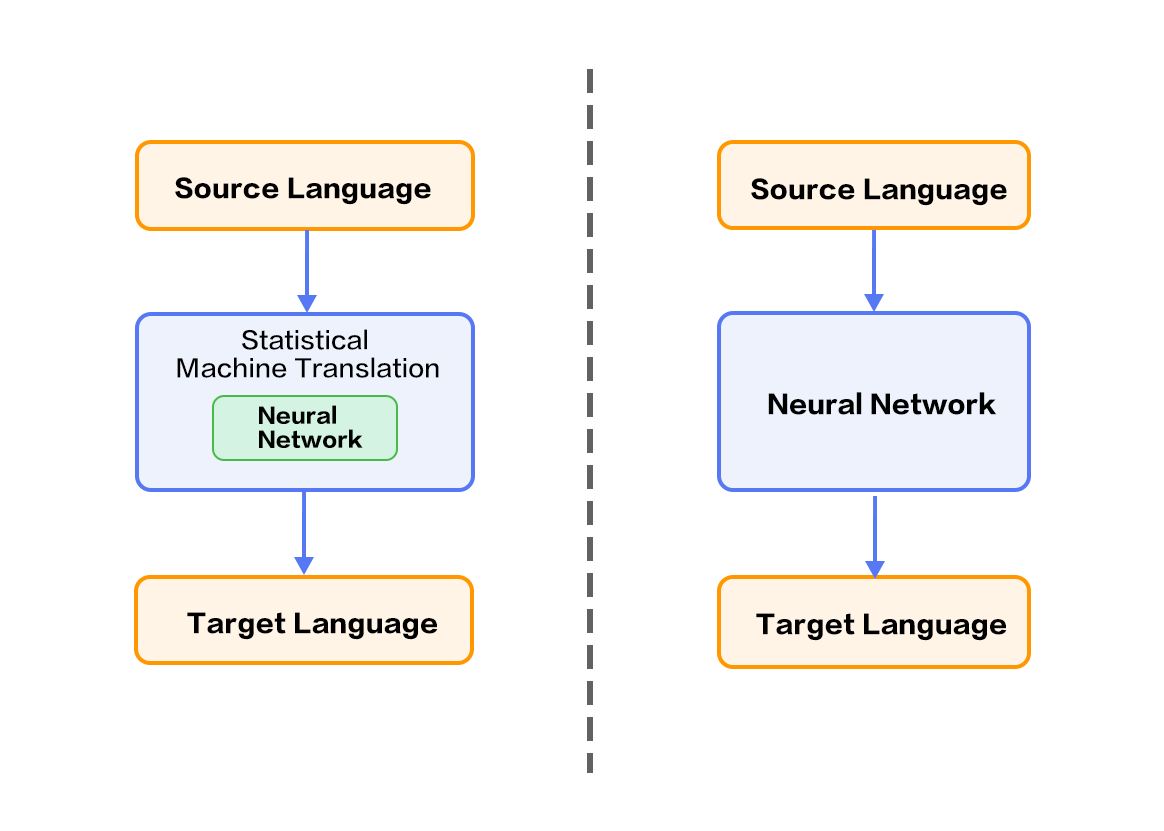The two main categories for deep learning based machine translation techniques are: 1. Techniques based on the statistical machine translation system but with some key components improved with neural networks, e.g., language model, reordering model (please refer to the left part of Figure 1); 2. Techniques mapping from source language to target language directly using a neural network, or end-to-end neural machine translation (NMT).

Figure 1. Neural Network based Machine Translation

This tutorial will mainly introduce an NMT model and how to use PaddlePaddle to train it. ## Illustrative Results Let's consider an example of Chinese-to-English translation. The model is given the following segmented sentence in Chinese ```text 这些 是 希望 的 曙光 和 解脱 的 迹象 . ``` After training and with a beam-search size of 3, the generated translations are as follows: ```text 0 -5.36816 These are signs of hope and relief . 1 -6.23177 These are the light of hope and relief . 2 -7.7914 These are the light of hope and the relief of hope . ``` - The first column corresponds to the id of the generated sentence; the second column corresponds to the score of the generated sentence (in descending order), where a larger value indicates better quality; the last column corresponds to the generated sentence. - There are two special tokens: `` denotes the end of a sentence while `` denotes unknown word, i.e., a word not in the training dictionary. ## Overview of the Model This section will introduce Gated Recurrent Unit (GRU), Bi-directional Recurrent Neural Network, the Encoder-Decoder framework used in NMT, attention mechanism, as well as the beam search algorithm. ### Gated Recurrent Unit (GRU) We already introduced RNN and LSTM in the [Sentiment Analysis](https://github.com/PaddlePaddle/book/blob/develop/understand_sentiment/README.md) chapter. Compared to a simple RNN, the LSTM added memory cell, input gate, forget gate and output gate. These gates combined with the memory cell greatly improve the ability to handle long-term dependencies. GRU\[[2](#references)\] proposed by Cho et al is a simplified LSTM and an extension of a simple RNN. It is shown in the figure below. A GRU unit has only two gates: - reset gate: when this gate is closed, the history information is discarded, i.e., the irrelevant historical information has no effect on the future output. - update gate: it combines the input gate and the forget gate and is used to control the impact of historical information on the hidden output. The historical information is passed over when the update gate is close to 1.

Figure 2. A GRU Gate

Generally speaking, sequences with short distance dependencies will have an active reset gate while sequences with long distance dependency will have an active update date. In addition, Chung et al.\[[3](#references)\] have empirically shown that although GRU has less parameters, it has similar performance to LSTM on several different tasks. ### Bi-directional Recurrent Neural Network We already introduced an instance of bi-directional RNN in the [Semantic Role Labeling](https://github.com/PaddlePaddle/book/blob/develop/label_semantic_roles/README.md) chapter. Here we present another bi-directional RNN model with a different architecture proposed by Bengio et al. in \[[2](#references),[4](#references)\]. This model takes a sequence as input and outputs a fixed dimensional feature vector at each step, encoding the context information at the corresponding time step. 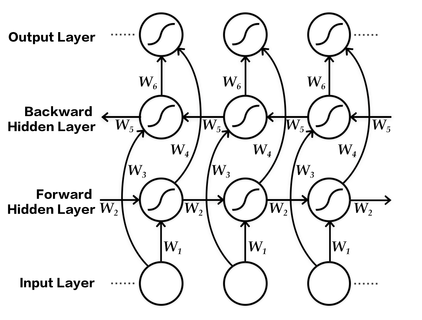Specifically, this bi-directional RNN processes the input sequence in the original and reverse order respectively, and then concatenates the output feature vectors at each time step as the final output. Thus the output node at each time step contains information from the past and future as context. The figure below shows an unrolled bi-directional RNN. This network contains a forward RNN and backward RNN with six weight matrices: weight matrices from input to forward hidden layer and backward hidden ($W_1, W_3$), weight matrices from hidden to itself ($W_2, W_5$), matrices from forward hidden and backward hidden to output layer ($W_4, W_6$). Note that there are no connections between forward hidden and backward hidden layers.

Figure 3. Temporally unrolled bi-directional RNN

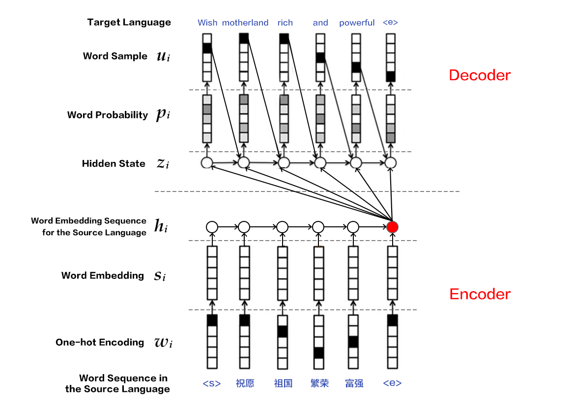
### Encoder-Decoder Framework The Encoder-Decoder\[[2](#references)\] framework aims to solve the mapping of a sequence to another sequence, for sequences with arbitrary lengths. The source sequence is encoded into a vector via an encoder, which is then decoded to a target sequence via a decoder by maximizing the predictive probability. Both the encoder and the decoder are typically implemented via RNN.

Figure 4. Encoder-Decoder Framework

#### Encoder There are three steps for encoding a sentence: 1. One-hot vector representation of a word: Each word $x_i$ in the source sentence $x=\left \{ x_1,x_2,...,x_T \right \}$ is represented as a vector $w_i\epsilon \left \{ 0,1 \right \}^{\left | V \right |},i=1,2,...,T$ where $w_i$ has the same dimensionality as the size of the dictionary, i.e., $\left | V \right |$, and has an element of one at the location corresponding to the location of the word in the dictionary and zero elsewhere. 2. Word embedding as a representation in the low-dimensional semantic space: There are two problems with one-hot vector representation * The dimensionality of the vector is typically large, leading to the curse of dimensionality; * It is hard to capture the relationships between words, i.e., semantic similarities. Therefore, it is useful to project the one-hot vector into a low-dimensional semantic space as a dense vector with fixed dimensions, i.e., $s_i=Cw_i$ for the $i$-th word, with $C\epsilon R^{K\times \left | V \right |}$ as the projection matrix and $K$ is the dimensionality of the word embedding vector. 3. Encoding of the source sequence via RNN: This can be described mathematically as: $$h_i=\varnothing _\theta \left ( h_{i-1}, s_i \right )$$ where $h_0$ is a zero vector, $\varnothing _\theta$ is a non-linear activation function, and $\mathbf{h}=\left \{ h_1,..., h_T \right \}$ is the sequential encoding of the first $T$ words from the source sequence. The vector representation of the whole sentence can be represented as the encoding vector at the last time step $T$ from $\mathbf{h}$, or by temporal pooling over $\mathbf{h}$. 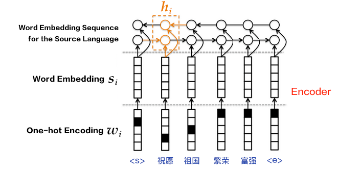Bi-directional RNN can also be used in step (3) for more a complicated sentence encoding. This can be implemented using a bi-directional GRU. Forward GRU encodes the source sequence in its original order $(x_1,x_2,...,x_T)$, and generates a sequence of hidden states $(\overrightarrow{h_1},\overrightarrow{h_2},...,\overrightarrow{h_T})$. The backward GRU encodes the source sequence in reverse order, i.e., $(x_T,x_T-1,...,x_1)$ and generates $(\overleftarrow{h_1},\overleftarrow{h_2},...,\overleftarrow{h_T})$. Then for each word $x_i$, its complete hidden state is the concatenation of the corresponding hidden states from the two GRUs, i.e., $h_i=\left [ \overrightarrow{h_i^T},\overleftarrow{h_i^T} \right ]^{T}$.

Figure 5. Encoder using bi-directional GRU

#### Decoder The goal of the decoder is to maximize the probability of the next correct word in the target language. The main idea is as follows: 1. At each time step $i$, given the encoding vector (or context vector) $c$ of the source sentence, the $i$-th word $u_i$ from the ground-truth target language and the RNN hidden state $z_i$, the next hidden state $z_{i+1}$ is computed as: $$z_{i+1}=\phi _{\theta '}\left ( c,u_i,z_i \right )$$ where $\phi _{\theta '}$ is a non-linear activation function and $c=q\mathbf{h}$ is the context vector of the source sentence. Without using [attention](#Attention Mechanism), if the output of the [encoder](#Encoder) is the encoding vector at the last time step of the source sentence, then $c$ can be defined as $c=h_T$. $u_i$ denotes the $i$-th word from the target language sentence and $u_0$ denotes the beginning of the target language sentence (i.e., ``), indicating the beginning of decoding. $z_i$ is the RNN hidden state at time step $i$ and $z_0$ is an all zero vector. 2. Calculate the probability $p_{i+1}$ for the $i+1$-th word in the target language sequence by normalizing $z_{i+1}$ using `softmax` as follows $$p\left ( u_{i+1}|u_{<i+1},\mathbf{x} \right )=softmax(W_sz_{i+1}+b_z)$$ where $W_sz_{i+1}+b_z$ scores each possible words and is then normalized via softmax to produce the probability $p_{i+1}$ for the $i+1$-th word. 3. Compute the cost accoding to $p_{i+1}$ and $u_{i+1}$. 4. Repeat Steps 1-3, until all the words in the target language sentence have been processed. The generation process of machine translation is to translate the source sentence into a sentence in the target language according to a pre-trained model. There are some differences between the decoding step in generation and training. Please refer to [Beam Search Algorithm](#Beam Search Algorithm) for details. 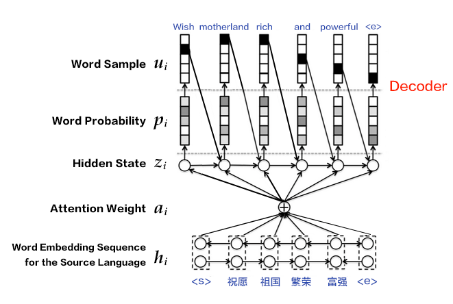### Attention Mechanism There are a few problems with the fixed dimensional vector representation from the encoding stage: * It is very challenging to encode both the semantic and syntactic information a sentence with a fixed dimensional vector regardless of the length of the sentence. * Intuitively, when translating a sentence, we typically pay more attention to the parts in the source sentence more relevant to the current translation. Moreover, the focus changes along the process of the translation. With a fixed dimensional vector, all the information from the source sentence is treated equally in terms of attention. This is not reasonable. Therefore, Bahdanau et al. \[[4](#references)\] introduced attention mechanism, which can decode based on different fragments of the context sequence in order to address the difficulty of feature learning for long sentences. Decoder with attention will be explained in the following. Different from the simple decoder, $z_i$ is computed as: $$z_{i+1}=\phi _{\theta '}\left ( c_i,u_i,z_i \right )$$ It is observed that for each word $u_i$ in the target language sentence, there is a corresponding context vector $c_i$ as the encoding of the source sentence, which is computed as: $$c_i=\sum _{j=1}^{T}a_{ij}h_j, a_i=\left[ a_{i1},a_{i2},...,a_{iT}\right ]$$ It is noted that the attention mechanism is achieved by a weighted average over the RNN hidden states $h_j$. The weight $a_{ij}$ denotes the strength of attention of the $i$-th word in the target language sentence to the $j$-th word in the source sentence and is calculated as $$a_{ij} = {exp(e_{ij}) \over {\sum_{k=1}^T exp(e_{ik})}}$$ $$e_{ij} = {align(z_i, h_j)}$$ where $align$ is an alignment model that measures the fitness between the $i$-th word in the target language sentence and the $j$-th word in the source sentence. More concretely, the fitness is computed with the $i$-th hidden state $z_i$ of the decoder RNN and the $j$-th context vector $h_j$ of the source sentence. Hard alignment is used in the conventional alignment model, which means each word in the target language explicitly corresponds to one or more words from the target language sentence. In an attention model, soft alignment is used, where any word in source sentence is related to any word in the target language sentence, where the strength of the relation is a real number computed via the model, thus can be incorporated into the NMT framework and can be trained via back-propagation.

Figure 6. Decoder with Attention Mechanism

### Beam Search Algorithm [Beam Search](http://en.wikipedia.org/wiki/Beam_search) is a heuristic search algorithm that explores a graph by expanding the most promising node in a limited set. It is typically used when the solution space is huge (e.g., for machine translation, speech recognition), and there is not enough memory for all the possible solutions. For example, if we want to translate “`你好`” into English, even if there are only three words in the dictionary (``, ``, `hello`), it is still possible to generate an infinite number of sentences, where the word `hello` can appear different number of times. Beam search could be used to find a good translation among them. Beam search builds a search tree using breadth first search and sorts the nodes according to a heuristic cost (sum of the log probability of the generated words) at each level of the tree. Only a fixed number of nodes according to the pre-specified beam size (or beam width) are considered. Thus, only nodes with highest scores are expanded in the next level. This reduces the space and time requirements significantly. However, a globally optimal solution is not guaranteed. The goal is to maximize the probability of the generated sequence when using beam search in decoding, The procedure is as follows: 1. At each time step $i$, compute the hidden state $z_{i+1}$ of the next time step according to the context vector $c$ of the source sentence, the $i$-th word $u_i$ generated for the target language sentence and the RNN hidden state $z_i$. 2. Normalize $z_{i+1}$ using `softmax` to get the probability $p_{i+1}$ for the $i+1$-th word for the target language sentence. 3. Sample the word $u_{i+1}$ according to $p_{i+1}$. 4. Repeat Steps 1-3, until end-of-sentence token `` is generated or the maximum length of the sentence is reached. Note: $z_{i+1}$ and $p_{i+1}$ are computed the same way as in [Decoder](#Decoder). In generation mode, each step is greedy in so there is no guarantee of a global optimum. ## BLEU Score Bilingual Evaluation understudy (BLEU) is a metric widely used for automatic machine translation proposed by IBM Watson Research Center in 2002\[[5](#References)\]. The closer the translation produced by a machine is to the translation produced by a human expert, the better the performance of the translation system. To measure the closeness between machine translation and human translation, sentence precision is used. It compares the number of matched n-grams. More matches will lead to higher BLEU scores. ## Data Preparation This tutorial uses a dataset from [WMT-14](http://www-lium.univ-lemans.fr/~schwenk/cslm_joint_paper/), where [bitexts (after selection)](http://www-lium.univ-lemans.fr/~schwenk/cslm_joint_paper/data/bitexts.tgz) is used as the training set, and [dev+test data](http://www-lium.univ-lemans.fr/~schwenk/cslm_joint_paper/data/dev+test.tgz) is used as test and generation set. ### Data Preprocessing There are two steps for pre-processing: - Merge the source and target parallel corpus files into one file - Merge `XXX.src` and `XXX.trg` file pair as `XXX` - The $i$-th row in `XXX` is the concatenation of the $i$-th row from `XXX.src` with the $i$-th row from `XXX.trg`, separated with '\t'. - Create source dictionary and target dictionary, each containing **DICTSIZE** number of words, including the most frequent (DICTSIZE - 3) fo word from the corpus and 3 special token `` (begin of sequence), `` (end of sequence) and `` (unknown words that are not in the vocabulary). ### A Subset of Dataset Because the full dataset is very big, to reduce the time for downloading the full dataset. PadddlePaddle package `paddle.dataset.wmt14` provides a preprocessed `subset of dataset`(http://paddlepaddle.bj.bcebos.com/demo/wmt_shrinked_data/wmt14.tgz). This subset has 193319 instances of training data and 6003 instances of test data. Dictionary size is 30000. Because of the limitation of size of the subset, the effectiveness of trained model from this subset is not guaranteed. ## Training Instructions ### Initialize PaddlePaddle ```python import sys import paddle.v2 as paddle # train with a single CPU paddle.init(use_gpu=False, trainer_count=1) # False: training, True: generating is_generating = False ``` ### Model Configuration 1. Define some global variables ```python dict_size = 30000 # dict dim source_dict_dim = dict_size # source language dictionary size target_dict_dim = dict_size # destination language dictionary size word_vector_dim = 512 # word embedding dimension encoder_size = 512 # hidden layer size of GRU in encoder decoder_size = 512 # hidden layer size of GRU in decoder beam_size = 3 # expand width in beam search max_length = 250 # a stop condition of sequence generation ``` 2. Implement Encoder as follows: - Input is a sequence of words represented by an integer word index sequence. So we define data layer of data type `integer_value_sequence`. The value range of each element in the sequence is `[0, source_dict_dim)` ```python src_word_id = paddle.layer.data( name='source_language_word', type=paddle.data_type.integer_value_sequence(source_dict_dim)) ``` - Map the one-hot vector (represented by word index) into a word vector $\mathbf{s}$ in a low-dimensional semantic space ```python src_embedding = paddle.layer.embedding( input=src_word_id, size=word_vector_dim) ``` - Use bi-direcitonal GRU to encode the source language sequence, and concatenate the encoding outputs from the two GRUs to get $\mathbf{h}$ ```python src_forward = paddle.networks.simple_gru( input=src_embedding, size=encoder_size) src_backward = paddle.networks.simple_gru( input=src_embedding, size=encoder_size, reverse=True) encoded_vector = paddle.layer.concat(input=[src_forward, src_backward]) ``` 3. Implement Attention-based Decoder as follows: - Get a projection of the encoding (c.f. 2.3) of the source language sequence by passing it into a feed forward neural network ```python encoded_proj = paddle.layer.fc( act=paddle.activation.Linear(), size=decoder_size, bias_attr=False, input=encoded_vector) ``` - Use a non-linear transformation of the last hidden state of the backward GRU on the source language sentence as the initial state of the decoder RNN $c_0=h_T$ ```python backward_first = paddle.layer.first_seq(input=src_backward) decoder_boot = paddle.layer.fc( size=decoder_size, act=paddle.activation.Tanh(), bias_attr=False, input=backward_first) ``` - Define the computation in each time step for the decoder RNN, i.e., according to the current context vector $c_i$, hidden state for the decoder $z_i$ and the $i$-th word $u_i$ in the target language to predict the probability $p_{i+1}$ for the $i+1$-th word. - decoder_mem records the hidden state $z_i$ from the previous time step, with an initial state as decoder_boot. - context is computed via `simple_attention` as $c_i=\sum {j=1}^{T}a_{ij}h_j$, where enc_vec is the projection of $h_j$ and enc_proj is the projection of $h_j$ (c.f. 3.1). $a_{ij}$ is calculated within `simple_attention`. - decoder_inputs fuse $c_i$ with the representation of the current_word (i.e., $u_i$). - gru_step uses `gru_step_layer` function to compute $z_{i+1}=\phi _{\theta '}\left ( c_i,u_i,z_i \right )$. - Softmax normalization is used in the end to computed the probability of words, i.e., $p\left ( u_i|u_{<i},\mathbf{x} \right )=softmax(W_sz_i+b_z)$. The output is returned. ```python def gru_decoder_with_attention(enc_vec, enc_proj, current_word): decoder_mem = paddle.layer.memory( name='gru_decoder', size=decoder_size, boot_layer=decoder_boot) context = paddle.networks.simple_attention( encoded_sequence=enc_vec, encoded_proj=enc_proj, decoder_state=decoder_mem) decoder_inputs = paddle.layer.fc( act=paddle.activation.Linear(), size=decoder_size * 3, bias_attr=False, input=[context, current_word], layer_attr=paddle.attr.ExtraLayerAttribute( error_clipping_threshold=100.0)) gru_step = paddle.layer.gru_step( name='gru_decoder', input=decoder_inputs, output_mem=decoder_mem, size=decoder_size) out = paddle.layer.fc( size=target_dict_dim, bias_attr=True, act=paddle.activation.Softmax(), input=gru_step) return out ``` 4. Define the name for the decoder and the first two input for `gru_decoder_with_attention`. Note that `StaticInput` is used for the two inputs. Please refer to [StaticInput Document](https://github.com/PaddlePaddle/Paddle/blob/develop/doc/v2/howto/rnn/recurrent_group_en.md#input) for more details. ```python decoder_group_name = "decoder_group" group_input1 = paddle.layer.StaticInput(input=encoded_vector) group_input2 = paddle.layer.StaticInput(input=encoded_proj) group_inputs = [group_input1, group_input2] ``` 5. Training mode: - Word embedding from the target language trg_embedding is passed to `gru_decoder_with_attention` as current_word. - `recurrent_group` calls `gru_decoder_with_attention` in a recurrent way - The sequence of next words from the target language is used as label (lbl) - Multi-class cross-entropy (`classification_cost`) is used to calculate the cost ```python if not is_generating: trg_embedding = paddle.layer.embedding( input=paddle.layer.data( name='target_language_word', type=paddle.data_type.integer_value_sequence(target_dict_dim)), size=word_vector_dim, param_attr=paddle.attr.ParamAttr(name='_target_language_embedding')) group_inputs.append(trg_embedding) # For decoder equipped with attention mechanism, in training, # target embeding (the groudtruth) is the data input, # while encoded source sequence is accessed to as an unbounded memory. # Here, the StaticInput defines a read-only memory # for the recurrent_group. decoder = paddle.layer.recurrent_group( name=decoder_group_name, step=gru_decoder_with_attention, input=group_inputs) lbl = paddle.layer.data( name='target_language_next_word', type=paddle.data_type.integer_value_sequence(target_dict_dim)) cost = paddle.layer.classification_cost(input=decoder, label=lbl) ``` 6. Generating mode: - The decoder predicts a next target word based on the the last generated target word. Embedding of the last generated word is automatically gotten by GeneratedInputs. - `beam_search` calls `gru_decoder_with_attention` in a recurrent way, to predict sequence id. ```python if is_generating: # In generation, the decoder predicts a next target word based on # the encoded source sequence and the previous generated target word. # The encoded source sequence (encoder's output) must be specified by # StaticInput, which is a read-only memory. # Embedding of the previous generated word is automatically retrieved # by GeneratedInputs initialized by a start mark . trg_embedding = paddle.layer.GeneratedInput( size=target_dict_dim, embedding_name='_target_language_embedding', embedding_size=word_vector_dim) group_inputs.append(trg_embedding) beam_gen = paddle.layer.beam_search( name=decoder_group_name, step=gru_decoder_with_attention, input=group_inputs, bos_id=0, eos_id=1, beam_size=beam_size, max_length=max_length) ``` Note: Our configuration is based on Bahdanau et al. \[[4](#references)\] but with a few simplifications. Please refer to [issue #1133](https://github.com/PaddlePaddle/Paddle/issues/1133) for more details. ## Model Training 1. Create Parameters Create every parameter that `cost` layer needs. And we can get parameter names. If the parameter name is not specified during model configuration, it will be generated. ```python if not is_generating: parameters = paddle.parameters.create(cost) for param in parameters.keys(): print param ``` 2. Define DataSet Create [**data reader**](https://github.com/PaddlePaddle/Paddle/tree/develop/doc/design/reader#python-data-reader-design-doc) for WMT-14 dataset. ```python if not is_generating: wmt14_reader = paddle.batch( paddle.reader.shuffle( paddle.dataset.wmt14.train(dict_size=dict_size), buf_size=8192), batch_size=5) ``` 3. Create trainer We need to tell trainer what to optimize, and how to optimize. Here trainer will optimize `cost` layer using stochastic gradient descent (SDG). ```python if not is_generating: optimizer = paddle.optimizer.Adam( learning_rate=5e-5, regularization=paddle.optimizer.L2Regularization(rate=8e-4)) trainer = paddle.trainer.SGD(cost=cost, parameters=parameters, update_equation=optimizer) ``` 4. Define event handler The event handler is a callback function invoked by trainer when an event happens. Here we will print log in event handler. ```python if not is_generating: def event_handler(event): if isinstance(event, paddle.event.EndIteration): if event.batch_id % 2 == 0: print "\nPass %d, Batch %d, Cost %f, %s" % ( event.pass_id, event.batch_id, event.cost, event.metrics) ``` 5. Start training ```python if not is_generating: trainer.train( reader=wmt14_reader, event_handler=event_handler, num_passes=2) ``` The training log is as follows: ```text Pass 0, Batch 0, Cost 247.408008, {'classification_error_evaluator': 1.0} Pass 0, Batch 10, Cost 212.058789, {'classification_error_evaluator': 0.8737863898277283} ... ``` ## Model Usage 1. Download Pre-trained Model As the training of an NMT model is very time consuming, we provide a pre-trained model. The model is trained with a cluster of 50 physical nodes (each node has two 6-core CPU) over 5 days. The provided model has the [BLEU Score](#BLEU Score) of 26.92, and the size of 205M. ```python if is_generating: parameters = paddle.dataset.wmt14.model() ``` 2. Define DataSet Get the first 3 samples of wmt14 generating set as the source language sequences. ```python if is_generating: gen_creator = paddle.dataset.wmt14.gen(dict_size) gen_data = [] gen_num = 3 for item in gen_creator(): gen_data.append((item[0], )) if len(gen_data) == gen_num: break ``` 3. Create infer Use inference interface `paddle.infer` return the prediction probability (see field `prob`) and labels (see field `id`) of each generated sequence. ```python if is_generating: beam_result = paddle.infer( output_layer=beam_gen, parameters=parameters, input=gen_data, field=['prob', 'id']) ``` 4. Print generated translation Print sequence and its `beam_size` generated translation results based on the dictionary. ```python if is_generating: # load the dictionary src_dict, trg_dict = paddle.dataset.wmt14.get_dict(dict_size) gen_sen_idx = np.where(beam_result[1] == -1)[0] assert len(gen_sen_idx) == len(gen_data) * beam_size # -1 is the delimiter of generated sequences. # the first element of each generated sequence its length. start_pos, end_pos = 1, 0 for i, sample in enumerate(gen_data): print(" ".join([src_dict[w] for w in sample[0][1:-1]])) for j in xrange(beam_size): end_pos = gen_sen_idx[i * beam_size + j] print("%.4f\t%s" % (beam_result[0][i][j], " ".join( trg_dict[w] for w in beam_result[1][start_pos:end_pos]))) start_pos = end_pos + 2 print("\n") ``` The generating log is as follows: ```text Les se au sujet de la largeur des sièges alors que de grosses commandes sont en jeu -19.0196 The will be rotated about the width of the seats , while large orders are at stake . -19.1131 The will be rotated about the width of the seats , while large commands are at stake . -19.5129 The will be rotated about the width of the seats , while large commands are at play . ``` ## Summary End-to-end neural machine translation is a recently developed way to perform machine translations. In this chapter, we introduced the typical "Encoder-Decoder" framework and "attention" mechanism. Since NMT is a typical Sequence-to-Sequence (Seq2Seq) learning problem, tasks such as query rewriting, abstraction generation, and single-turn dialogues can all be solved with the model presented in this chapter. ## References 1. Koehn P. [Statistical machine translation](https://books.google.com.hk/books?id=4v_Cx1wIMLkC&printsec=frontcover&hl=zh-CN&source=gbs_ge_summary_r&cad=0#v=onepage&q&f=false)[M]. Cambridge University Press, 2009. 2. Cho K, Van Merriënboer B, Gulcehre C, et al. [Learning phrase representations using RNN encoder-decoder for statistical machine translation](http://www.aclweb.org/anthology/D/D14/D14-1179.pdf)[C]//Proceedings of the 2014 Conference on Empirical Methods in Natural Language Processing (EMNLP), 2014: 1724-1734. 3. Chung J, Gulcehre C, Cho K H, et al. [Empirical evaluation of gated recurrent neural networks on sequence modeling](https://arxiv.org/abs/1412.3555)[J]. arXiv preprint arXiv:1412.3555, 2014. 4. Bahdanau D, Cho K, Bengio Y. [Neural machine translation by jointly learning to align and translate](https://arxiv.org/abs/1409.0473)[C]//Proceedings of ICLR 2015, 2015. 5. Papineni K, Roukos S, Ward T, et al. [BLEU: a method for automatic evaluation of machine translation](http://dl.acm.org/citation.cfm?id=1073135)[C]//Proceedings of the 40th annual meeting on association for computational linguistics. Association for Computational Linguistics, 2002: 311-318.
This tutorial is contributed by PaddlePaddle, and licensed under a Creative Commons Attribution-ShareAlike 4.0 International License.