Design Doc: Computations as Graphs
A primary goal of the refactorization of PaddlePaddle is a more flexible representation of deep learning computation, in particular, a graph of operators and variables, instead of sequences of layers as before.
This document explains that the construction of a graph as three steps:
- construct the forward part
- construct the backward part
- construct the optimization part
Let us take the problem of image classification as a simple example. The application program that trains the model looks like:
x = layer.data("images")
l = layer.data("label")
y = layer.fc(x)
cost = layer.mse(y, l)
optimize(cost)
train(cost, reader=mnist.train())
Forward Part
The first four lines of above program build the forward part of the graph.

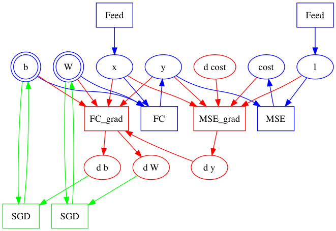
In particular, the first line x = layer.data("images") creates variable x and a Feed operator that copies a column from the minibatch to x. y = layer.fc(x) creates not only the FC operator and output variable y, but also two parameters, W and b.
In this example, all operators are created as OpDesc protobuf messages, and all variables are VarDesc. These protobuf messages are saved in a BlockDesc protobuf message.
Backward Part
The fifth line optimize(cost) calls two functions, ConstructBackwardGraph and ConstructOptimizationGraph.
ConstructBackwardGraph traverses the forward graph in the BlockDesc protobuf message and builds the backward part.

According to the chain rule of gradient computation, ConstructBackwardGraph would
- create a gradient operator G for each operator F,
- make all inputs, outputs, and outputs’ gradient of F as inputs of G,
- create gradients for all inputs of F, except for those who don’t have gradients, like x and l, and
- make all these gradients as outputs of G.
Optimization Part
For each parameter, like W and b created by layer.fc, marked as double circles in above graphs, ConstructOptimizationGraph creates an optimization operator to apply its gradient. Here results in the complete graph:

