# Word Vector
The source code of this tutorial is in [book/word2vec](https://github.com/PaddlePaddle/book/tree/develop/04.word2vec). For new users, please refer to [Running This Book](https://github.com/PaddlePaddle/book/blob/develop/README.md#running-the-book) .
## Background
In this chapter, we'll introduce the vector representation of words, also known as word embedding. Word vector is a common operation in natural language processing. It is a common technology underlying Internet services such as search engines, advertising systems, and recommendation systems.
In these Internet services, we often compare the correlation between two words or two paragraphs of text. In order to make such comparisons, we often have to express words in a way that is suitable for computer processing. The most natural way is probably the vector space model.In this way, each word is represented as a one-hot vector whose length is the dictionary size, and each dimension corresponds to each word in a dictionary, except that the value in the corresponding dimension of the word is 1, other elements are 0.
The One-hot vector is natural but has limitation. For example, in the internet advertising system, if the query entered by the user is "Mother's Day", the keyword of an advertisement is "Carnation". Although according to common sense, we know that there is a connection between these two words - Mother's Day should usually give the mother a bunch of carnations; but the distance between the two words corresponds to the one-hot vectors, whether it is Euclidean distance or cosine similarity, the two words are considered to be irrelevant due to their vector orthogonality. The root cause of this conclusion contradicting us is that the amount of information in each word itself is too small. Therefore, just giving two words is not enough for us to accurately determine whether they are relevant. To accurately calculate correlations, we need more information—knowledge from a large amount of data through machine learning methods.
In the field of machine learning, all kinds of "knowledge" are represented by various models, and the word embedding model is one of them. A one-hot vector can be mapped to a lower-dimensional embedding vector by the word embedding model, such as $embedding (Mother's day) = [0.3, 4.2, -1.5, ...], embedding (carnation) = [0.2, 5.6, -2.3, ...]$. In this representation of the embedding vector to which it is mapped, it is desirable that the word vectors corresponding to the similar words on the two semantics (or usages) are "more like", such that the cosine similarity of the corresponding word vectors of "Mother's Day" and "Carnation" is no longer zero.
The word embedding model can be a probability model, a co-occurrence matrix model, or a neural network model. Before implementing neural networks to calculate the embedding vector, the traditional method is to count the co-occurrence matrix $X$ of a word. $X$ is a matrix of $|V| \times |V|$ size, $X_{ij}$ means that in all corpora, The number of words appearing simultaneously with the i-th word and the j-th word in the vocabulary $V$(vocabulary), $|V|$ is the size of the vocabulary. Do matrix decomposition for $X$ (such as singular value decomposition, Singular Value Decomposition \[[5](#references)\]), and the result $U$ is treated as the embedding vector for all words:
$$X = USV^T$$
But such traditional method has many problems:
1) Since many words do not appear, the matrix is extremely sparse, so additional processing of the word frequency is needed to achieve a good matrix decomposition effect;
2) The matrix is very large and the dimensions are too high (usually up to $10^6 \times 10^6$);
3) You need to manually remove the stop words (such as although, a, ...), otherwise these frequently occurring words will also affect the effect of matrix decomposition.
The neural-network-based model does not need to calculate and store a large table that is statistically generated on the whole corpus, but obtains the word vector by learning the semantic information, so the problem above can be well solved. In this chapter, we will show the details of training word vectors based on neural networks and how to train a word embedding model with PaddlePaddle.
## Result Demo
In this chapter, after the embedding vector is trained, we can use the data visualization algorithm t-SNE\[[4](#references)\] to draw the projection of the word features in two dimensions (as shown below). As can be seen from the figure, semantically related words (such as a, the, these; big, huge) are very close in projection, and semantic unrelated words (such as say, business; decision, japan) are far away from the projection.

Figure 1. Two-dimensional projection of a word vector
On the other hand, we know that the cosine of two vectors is in the interval of $[-1,1]$: two identical vector cosines are 1, and the cosine value between two mutually perpendicular vectors is 0, The vector cosine of the opposite direction is -1, which the correlation is proportional to the magnitude of the cosine. So we can also calculate the cosine similarity of two word vectors:
```
please input two words: big huge
Similarity: 0.899180685161
please input two words: from company
Similarity: -0.0997506977351
```
The results above can be obtained by running `calculate_dis.py`, loading the words in the dictionary and the corresponding training feature results. We will describe the usage for details in [model application](#model application).
## Overview of Models
Here we introduce three models of training word vectors: N-gram model, CBOW model and Skip-gram model. Their central idea is to get the probability of a word appearing through the context. For the N-gram model, we will first introduce the concept of the language model. In the section [training model](#training model), we'll tutor you to implement it with PaddlePaddle. The latter two models are the most famous neuron word vector models in recent years, developed by Tomas Mikolov in Google \[[3](#references)\], although they are very simple, but the training effect is very good.
### Language Model
Before introducing the word embedding model, let us introduce a concept: the language model.
The language model is intended to model the joint probability function $P(w_1, ..., w_T)$ of a sentence, where $w_i$ represents the ith word in the sentence. The goal of the language model isn that the model gives a high probability to meaningful sentences and a small probability to meaningless sentences.Such models can be applied to many fields, such as machine translation, speech recognition, information retrieval, part-of-speech tagging, handwriting recognition, etc., All of which hope to obtain the probability of a continuous sequence. Take information retrieval as an example, when you search for "how long is a football bame" (bame is a medical term), the search engine will prompt you if you want to search for "how long is a football game", because the probability of calculating "how long is a football bame" is very low, and the word is similar to bame, which may cause errors, the game will maximize the probability of generating the sentence.
For the target probability of the language model $P(w_1, ..., w_T)$, if it is assumed that each word in the text is independent, the joint probability of the whole sentence can be expressed as the product of the conditional probabilities of all the words. which is:
$$P(w_1, ..., w_T) = \prod_{t=1}^TP(w_t)$$
However, we know that the probability of each word in the statement is closely related to the word in front of it, so in fact, the language model is usually represented by conditional probability:
$$P(w_1, ..., w_T) = \prod_{t=1}^TP(w_t | w_1, ... , w_{t-1})$$
### N-gram neural model
In computational linguistics, n-gram is an important text representation method that represents a continuous n items in a text. Each item can be a letter, word or syllable based on the specific application scenario. The n-gram model is also an important method in the statistical language model. When n-gram is used to train the language model, the nth word is generally predicted by the content of the n-1 words of each n-gram.
Scientists such as Yoshua Bengio introduced how to learn a word vector model of a neural network representation in the famous paper Neural Probabilistic Language Models \[[1](#references)\ in 2003. The Neural Network Language Model (NNLM) in this paper connects the linear model and a nonlinear hidden layer. It learns the language model and the word vector simultaneously, that is, by learning a large number of corpora to obtain the vector expression of the words, and the probability of the entire sentence is obtained by using these vectors. Since all words are represented by a low-dimensional vector, learning the language model in this way can overcome the curse of dimensionality.
Note: Because the "Neural Network Language Model" is more general, we do not use the real name of NNLM here, considering its specific practice, this model here is called N-gram neural model.
We have already mentioned above using the conditional probability language model, that is, the probability of the $t$ word in a sentence is related to the first $t-1$ words of the sentence. The farther the word actually has the smaller effect on the word, then if you consider an n-gram, each word is only affected by the preceding `n-1` words, then:
$$P(w_1, ..., w_T) = \prod_{t=n}^TP(w_t|w_{t-1}, w_{t-2}, ..., w_{t-n+1 })$$
Given some real corpora, these corpora are meaningful sentences, and the optimization goal of the N-gram model is to maximize the objective function:
$$\frac{1}{T}\sum_t f(w_t, w_{t-1}, ..., w_{t-n+1};\theta) + R(\theta)$$
Where $f(w_t, w_{t-1}, ..., w_{t-n+1})$ represents the conditional probability of getting the current word $w_t$ based on historical n-1 words, $R(\theta )$ represents a parameter regularization item.

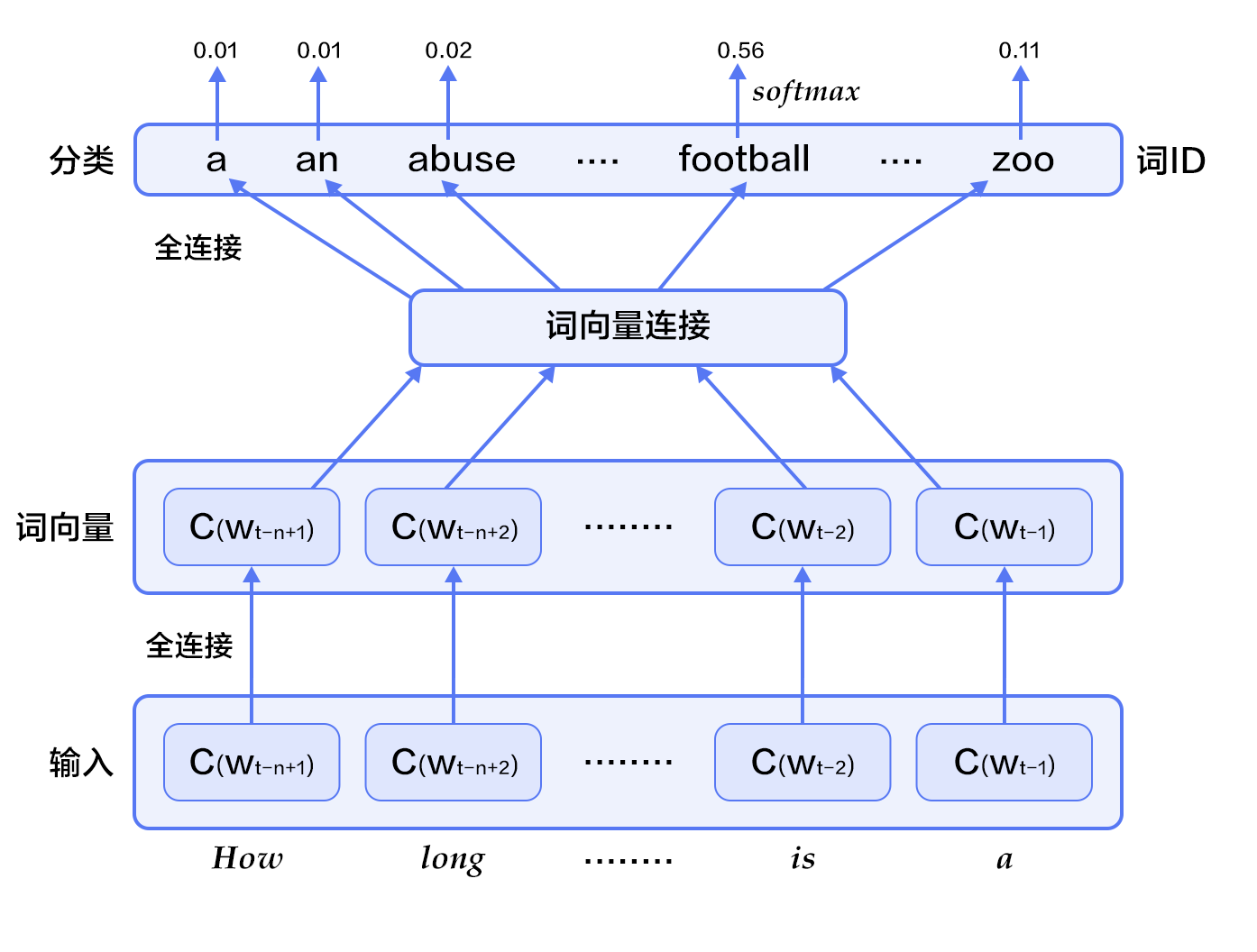
Figure 2. N-gram neural network model
Figure 2 shows the N-gram neural network model. From the bottom up, the model is divided into the following parts:
- For each sample, the model enters $w_{t-n+1},...w_{t-1}$, and outputs the probability distribution of the t-th word in the dictionary on the `|V|` words.
Each input word $w_{t-n+1},...w_{t-1}$ first maps to the word vector $C(w_{t-n+1}),...W_{t-1})$ by the mapping matrix.
- Then the word vectors of all words are spliced into a large vector, and a hidden layer representation of the historical words is obtained through a non-linear mapping:
$$g=Utanh(\theta^Tx + b_1) + Wx + b_2$$
Among them, $x$ is a large vector of all words, representing text history features; $\theta$, $U$, $b_1$, $b_2$, and $W$ are respectively parameters for the word vector layer to the hidden layer connection. $g$ represents the probability of all output words that are not normalized, and $g_i$ represents the output probability of the $i$ word in the unnormalized dictionary.
- According to the definition of softmax, by normalizing $g_i$, the probability of generating the target word $w_t$ is:
$$P(w_t | w_1, ..., w_{t-n+1}) = \frac{e^{g_{w_t}}}{\sum_i^{|V|} e^{g_i}}$$
- The loss value of the entire network is the multi-class classification cross entropy, which is expressed as
$$J(\theta) = -\sum_{i=1}^N\sum_{k=1}^{|V|}y_k^{i}log(softmax(g_k^i))$$
where $y_k^i$ represents the real label (0 or 1) of the $i$ sample of the $k$ class, and $softmax(g_k^i)$ represents the probability of the kth softmax output of the i-th sample.
### Continuous Bag-of-Words model(CBOW)
The CBOW model predicts the current word through the context of a word (each N words). When N=2, the model is shown below:

Figure 3. CBOW model
Specifically, regardless of the contextual word input order, CBOW uses the mean of the word vectors of the context words to predict the current word. which is:
$$context = \frac{x_{t-1} + x_{t-2} + x_{t+1} + x_{t+2}}{4}$$
Where $x_t$ is the word vector of the $t$th word, the score vector (score) $z=U\*context$, the final classification $y$ uses softmax, and the loss function uses multi-class classification cross entropy.
### Skip-gram model
The benefit of CBOW is that the distribution of contextual words is smoothed over the word vector, removing noise. Therefore it is very effective on small data sets. In the Skip-gram method, a word is used to predict its context, and many samples of the current word context are obtained, so it can be used for a larger data set.

Figure 4. Skip-gram model
As shown in the figure above, the specific method of the Skip-gram model is to map the word vector of a word to the word vector of $2n$ words ($2n$ represents the $n$ words before and after the input word), and then obtained the sum of the classification loss values of the $2n$ words by softmax.
## Data Preparation
### Data Introduction
This tutorial uses the Penn Treebank (PTB) (pre-processed version of Tomas Mikolov) dataset. The PTB data set is small and the training speed is fast. It is applied to Mikolov's open language model training tool \[[2](#references)\]. Its statistics are as follows:
| Training data |
Verify data |
Test data |
| ptb.train.txt |
ptb.valid.txt |
ptb.test.txt |
| 42068 sentences |
3370 sentences |
3761 sentence |
### Data Preprocessing
This chapter trains the 5-gram model, which means that the first 4 words of each piece of data are used to predict the 5th word during PaddlePaddle training. PaddlePaddle provides the python package `paddle.dataset.imikolov` corresponding to the PTB dataset, which automatically downloads and preprocesses the data for your convenience.
Preprocessing adds the start symbol `` and the end symbol `` to each sentence in the data set. Then, depending on the window size (5 in this tutorial), slide the window to the right each time from start to end and generate a piece of data.
For example, "I have a dream that one day" provides 5 pieces of data:
```text
I have a dream
I have a dream that
Have a dream that one
a dream that one day
Dream that one day
```
Finally, based on the position of its word in the dictionary, each input is converted to an index sequence of integers as the input to PaddlePaddle.
## Program the Model
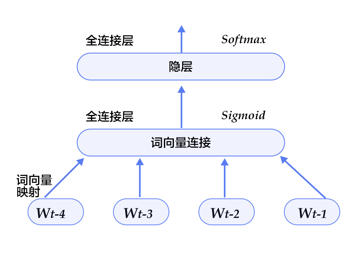
The model structure of this configuration is shown below:

Figure 5. N-gram neural network model in model configuration
First, load packages:
```python
from __future__ import print_function
import paddle
import paddle.fluid as fluid
import six
import numpy
import math
```
Then, define the parameters:
```python
EMBED_SIZE = 32 # embedding dimensions
HIDDEN_SIZE = 256 # hidden layer size
N = 5 # ngram size, here fixed 5
BATCH_SIZE = 100 # batch size
PASS_NUM = 100 # Training rounds
use_cuda = False # Set to True if trained with GPU
word_dict = paddle.dataset.imikolov.build_dict()
dict_size = len(word_dict)
```
A larger `BATCH_SIZE` will make the training converge faster, but it will also consume more memory. Since the word vector calculation is large, if the environment allows, please turn on the GPU for training, and get results faster.
Unlike the previous PaddlePaddle v2 version, in the new Fluid version, we don't have to manually calculate the word vector. PaddlePaddle provides a built-in method `fluid.embedding`, which we can use directly to construct an N-gram neural network.
- Let's define our N-gram neural network structure. This structure is used in both training and predicting. Because the word vector is sparse, we pass the parameter `is_sparse == True` to speed up the update of the sparse matrix.
```python
def inference_program(words, is_sparse):
embed_first = fluid.embedding(
input=words[0],
size=[dict_size, EMBED_SIZE],
dtype='float32',
is_sparse=is_sparse,
param_attr='shared_w')
embed_second = fluid.embedding(
input=words[1],
size=[dict_size, EMBED_SIZE],
dtype='float32',
is_sparse=is_sparse,
param_attr='shared_w')
embed_third = fluid.embedding(
input=words[2],
size=[dict_size, EMBED_SIZE],
dtype='float32',
is_sparse=is_sparse,
param_attr='shared_w')
embed_fourth = fluid.embedding(
input=words[3],
size=[dict_size, EMBED_SIZE],
dtype='float32',
is_sparse=is_sparse,
param_attr='shared_w')
concat_embed = fluid.layers.concat(
input=[embed_first, embed_second, embed_third, embed_fourth], axis=1)
hidden1 = fluid.layers.fc(input=concat_embed,
size=HIDDEN_SIZE,
act='sigmoid')
predict_word = fluid.layers.fc(input=hidden1, size=dict_size, act='softmax')
return predict_word
```
- Based on the neural network structure above, we can define our training method as follows:
```python
def train_program(predict_word):
# The definition of'next_word' must be after the declaration of inference_program.
# Otherwise the sequence of the train program input data becomes [next_word, firstw, secondw,
#thirdw, fourthw], This is not true.
next_word = fluid.data(name='nextw', shape=[None, 1], dtype='int64')
cost = fluid.layers.cross_entropy(input=predict_word, label=next_word)
avg_cost = fluid.layers.mean(cost)
return avg_cost
def optimizer_func():
return fluid.optimizer.AdagradOptimizer(
learning_rate=3e-3,
regularization=fluid.regularizer.L2DecayRegularizer(8e-4))
```
- Now we can start training. This version is much simpler than before. We have ready-made training and test sets: `paddle.dataset.imikolov.train()` and `paddle.dataset.imikolov.test()`. Both will return a reader. In PaddlePaddle, the reader is a Python function that reads the next piece of data when called each time . It is a Python generator.
`fluid.io.batch` will read in a reader and output a batched reader. We can also output the training of each step and batch during the training process.
```python
def train(if_use_cuda, params_dirname, is_sparse=True):
place = fluid.CUDAPlace(0) if if_use_cuda else fluid.CPUPlace()
train_reader = fluid.io.batch(
paddle.dataset.imikolov.train(word_dict, N), BATCH_SIZE)
test_reader = fluid.io.batch(
paddle.dataset.imikolov.test(word_dict, N), BATCH_SIZE)
first_word = fluid.data(name='firstw', shape=[None, 1], dtype='int64')
second_word = fluid.data(name='secondw', shape=[None, 1], dtype='int64')
third_word = fluid.data(name='thirdw', shape=[None, 1], dtype='int64')
forth_word = fluid.data(name='fourthw', shape=[None, 1], dtype='int64')
next_word = fluid.data(name='nextw', shape=[None, 1], dtype='int64')
word_list = [first_word, second_word, third_word, forth_word, next_word]
feed_order = ['firstw', 'secondw', 'thirdw', 'fourthw', 'nextw']
main_program = fluid.default_main_program()
star_program = fluid.default_startup_program()
predict_word = inference_program(word_list, is_sparse)
avg_cost = train_program(predict_word)
test_program = main_program.clone(for_test=True)
optimizer = optimizer_func()
optimizer.minimize(avg_cost)
exe = fluid.Executor(place)
def train_test(program, reader):
count = 0
feed_var_list = [
program.global_block().var(var_name) for var_name in feed_order
]
feeder_test = fluid.DataFeeder(feed_list=feed_var_list, place=place)
test_exe = fluid.Executor(place)
accumulated = len([avg_cost]) * [0]
for test_data in reader():
avg_cost_np = test_exe.run(
program=program,
feed=feeder_test.feed(test_data),
fetch_list=[avg_cost])
accumulated = [
x[0] + x[1][0] for x in zip(accumulated, avg_cost_np)
]
count += 1
return [x / count for x in accumulated]
def train_loop():
step = 0
feed_var_list_loop = [
main_program.global_block().var(var_name) for var_name in feed_order
]
feeder = fluid.DataFeeder(feed_list=feed_var_list_loop, place=place)
exe.run(star_program)
for pass_id in range(PASS_NUM):
for data in train_reader():
avg_cost_np = exe.run(
main_program, feed=feeder.feed(data), fetch_list=[avg_cost])
if step % 10 == 0:
outs = train_test(test_program, test_reader)
print("Step %d: Average Cost %f" % (step, outs[0]))
# The entire training process takes several hours if the average loss is less than 5.8,
# We think that the model has achieved good results and can stop training.
# Note 5.8 is a relatively high value, in order to get a better model, you can
# set the threshold here to be 3.5, but the training time will be longer.
if outs[0] < 5.8:
if params_dirname is not None:
fluid.io.save_inference_model(params_dirname, [
'firstw', 'secondw', 'thirdw', 'fourthw'
], [predict_word], exe)
return
step += 1
if math.isnan(float(avg_cost_np[0])):
sys.exit("got NaN loss, training failed.")
raise AssertionError("Cost is too large {0:2.2}".format(avg_cost_np[0]))
train_loop()
```
- `train_loop` will start training. The log of the training process during the period is as follows:
```text
Step 0: Average Cost 7.337213
Step 10: Average Cost 6.136128
Step 20: Average Cost 5.766995
...
```
## Model Application
After the model is trained, we can use it to make some predictions.
### Predict the next word
We can use our trained model to predict the next word after learning the previous N-gram.
```python
def infer(use_cuda, params_dirname=None):
place = fluid.CUDAPlace(0) if use_cuda else fluid.CPUPlace()
exe = fluid.Executor(place)
inference_scope = fluid.core.Scope()
with fluid.scope_guard(inference_scope):
#Get the inference program using fluid.io.load_inference_model,
#feed variable name by feed_target_names and fetch fetch_targets from scope
[inferencer, feed_target_names,
fetch_targets] = fluid.io.load_inference_model(params_dirname, exe)
# Set the input and use 4 LoDTensor to represent 4 words. Each word here is an id,
# Used to query the embedding table to get the corresponding word vector, so its shape size is [1].
# recursive_sequence_lengths sets the length based on LoD, so it should all be set to [[1]]
# Note that recursive_sequence_lengths is a list of lists
data1 = numpy.asarray([[211]], dtype=numpy.int64) # 'among'
data2 = numpy.asarray([[6]], dtype=numpy.int64) # 'a'
data3 = numpy.asarray([[96]], dtype=numpy.int64) # 'group'
data4 = numpy.asarray([[4]], dtype=numpy.int64) # 'of'
lod = numpy.asarray([[1]], dtype=numpy.int64)
first_word = fluid.create_lod_tensor(data1, lod, place)
second_word = fluid.create_lod_tensor(data2, lod, place)
third_word = fluid.create_lod_tensor(data3, lod, place)
fourth_word = fluid.create_lod_tensor(data4, lod, place)
assert feed_target_names[0] == 'firstw'
assert feed_target_names[1] == 'secondw'
assert feed_target_names[2] == 'thirdw'
assert feed_target_names[3] == 'fourthw'
# Construct the feed dictionary {feed_target_name: feed_target_data}
# Prediction results are included in results
results = exe.run(
inferencer,
feed={
feed_target_names[0]: first_word,
feed_target_names[1]: second_word,
feed_target_names[2]: third_word,
feed_target_names[3]: fourth_word
},
fetch_list=fetch_targets,
return_numpy=False)
print(numpy.array(results[0]))
most_possible_word_index = numpy.argmax(results[0])
print(most_possible_word_index)
print([
key for key, value in six.iteritems(word_dict)
if value == most_possible_word_index
][0])
```
Since the word vector matrix itself is relatively sparse, the training process takes a long time to reach a certain precision. In order to see the effect simply, the tutorial only sets up with a few rounds of training and ends with the following result. Our model predicts that the next word for `among a group of` is `the`. This is in line with the law of grammar. If we train for longer time, such as several hours, then the next predicted word we will get is `workers`. The format of the predicted output is as follows:
```text
[[0.03768077 0.03463154 0.00018074 ... 0.00022283 0.00029888 0.02967956]]
0
the
```
The first line represents the probability distribution of the predicted word in the dictionary, the second line represents the id corresponding to the word with the highest probability, and the third line represents the word with the highest probability.
The entrance to the entire program is simple:
```python
def main(use_cuda, is_sparse):
if use_cuda and not fluid.core.is_compiled_with_cuda():
return
params_dirname = "word2vec.inference.model"
train(
if_use_cuda=use_cuda,
params_dirname=params_dirname,
is_sparse=is_sparse)
infer(use_cuda=use_cuda, params_dirname=params_dirname)
main(use_cuda=use_cuda, is_sparse=True)
```
## Conclusion
In this chapter, we introduced word vectors, the relationship between language models and word vectors and how to obtain word vectors by training neural network models. In information retrieval, we can judge the correlation between query and document keywords based on the cosine value between vectors. In syntactic analysis and semantic analysis, trained word vectors can be used to initialize the model for better results. In the document classification, after the word vector, you can cluster to group synonyms in a document, or you can use N-gram to predict the next word. We hope that everyone can easily use the word vector to conduct research in related fields after reading this chapter.
## References
1. Bengio Y, Ducharme R, Vincent P, et al. [A neural probabilistic language model](http://www.jmlr.org/papers/volume3/bengio03a/bengio03a.pdf)[J]. journal of machine learning Research, 2003, 3(Feb): 1137-1155.
2. Mikolov T, Kombrink S, Deoras A, et al. [Rnnlm-recurrent neural network language modeling toolkit](http://www.fit.vutbr.cz/~imikolov/rnnlm/rnnlm-demo.pdf)[C ]//Proc. of the 2011 ASRU Workshop. 2011: 196-201.
3. Mikolov T, Chen K, Corrado G, et al. [Efficient estimation of word representations in vector space](https://arxiv.org/pdf/1301.3781.pdf)[J]. arXiv preprint arXiv:1301.3781, 2013 .
4. Maaten L, Hinton G. [Visualizing data using t-SNE](https://lvdmaaten.github.io/publications/papers/JMLR_2008.pdf)[J]. Journal of Machine Learning Research, 2008, 9(Nov ): 2579-2605.
5. https://en.wikipedia.org/wiki/Singular_value_decomposition

This tutorial is contributed by PaddlePaddle, and licensed under a Creative Commons Attribution-ShareAlike 4.0 International License.


