# Generative Adversarial Network The source code for this tutorial is in book/09.gan，For the first time to use , please refer to the instruction manual of the Book document. ### Description: ### 1. Hardware environment requirements: This article can support running under CPU and GPU 2. CUDA / cuDNN version supported by docker image: If docker is used to run book, please note that the GPU environment of the default image provided here is CUDA 8 / cuDNN 5. For GPUs requiring CUDA 9 such as NVIDIA Tesla V100, using this image may fail. 3. Consistency of code in documents and scripts: Please note: to make this article easier to read and use, we split and adjusted the code of dc_gan.py and put it in this article. The code in this article is consistent with the running result of dc_gan.py, which can be verified by running [train.py](https://github.com/PaddlePaddle/book/blob/develop/01.fit_a_line/train.py). ## Background GAN（Generative Adversarial Network \[[1](#Reference)\]，GAN for short） is a method of unsupervised learning, learn by two neural networks contest with each other in a game. This method was originally proposed by lan·Goodfellow and others in 2014. The origin paper is [Generative Adversarial Network](https://arxiv.org/abs/1406.2661)。 The Generative Adversarial Network consists of a generative network and a discriminative network. Using random sampling from the latent space as input, the output of the generative network needs to imitate the real samples in the training set as much as possible. The input of the discriminative network is the real sample or the output of the generative network. The purpose is to distinguish the output of the generative network from the real samples as much as possible. The two networks oppose each other and continuously adjust the parameters. The purpose is to distinguish the samples generated by the generative network from the real samples as much as possible\[[2](#References)\]. GAN is often used to generate fake images \[[3](#References)\] ）。In addition, the method is also used to reconstruct 3D models of objects from images, model patterns of motion in video and so on. 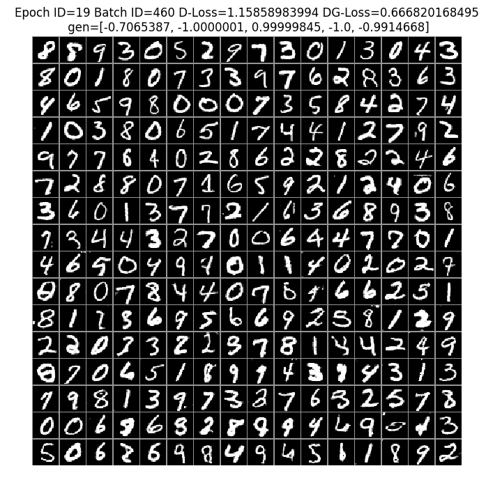## Result In this tutorial, we use MNIST data set as input for training. After 19 rounds of training, we can see that the generated image is very close to the the real image. In the following figure, the first 8 lines are the appearance of the real image, and the last 8 lines are the image generated by the network:

figure 1. handwritten number generated by GAN

## Model Overview ### GAN GAN is a way to learn the generative model of data distribution through adversarial methods. Among them, "Adversarial" refers to the mutual confrontation between Generator and Discriminator. Here, we will take the generated picture as an example to illustrate: - The generative network (G) receives a random noise z, and generates an image of approximate samples as much as possible, which is recorded as G(z) - The discriminative network (D) receives an input image x, and try to distinguish the image is a real sample or a false sample generated by the generative network. The output of the discriminative network is D(x) represents the probability that x is a real image. If D(x) = 1, it means that the discriminative network thinks the input must be a real image, if D(x) = 0, it means that the discriminative network thinks the input must be a false image. In the process of training, the two networks fight against each other and finally form a dynamic balance. The above process can be described by the formula as following:

In the best case, G can generate a image G(z), which is very similar to the real image, and it is difficult for D to judge whether the generated picture is true or not, and make a random guess on the true or false of the image, that is D(G(z))=0.5。 The following figure shows the training process of GAN. The real image distribution, generated image distribution and discriminative model are black line, green line and blue line respectively in the figure. At the beginning of training, the discriminative model can not distinguish the real images from the generated images. Then, when we fixed the generative model and optimize the discriminative model, the results are shown in the second figure. It can be seen that the discriminative model can distinguish the generated data from the real data. The third step is to fixed the discriminative model, optimize the generative model, and try to make the discriminative model unable to distinguish the generated images from the real images. In this process, it can be seen that the distribution of the images generated by the model is closer to the distribution of the real images. Such iterations continue until the final convergence, and the generated distribution and the real distribution coincide and the discriminative model cannot distinguish the real images from the generated images.

figure 2. GAN training process

But in the actual process, it is difficult to get this perfect equilibrium point, and the convergence theory of GAN is still in continuous research. ### DCGAN [DCGAN](https://arxiv.org/abs/1511.06434) \[[4](#Reference)\] is the combination of deep convolution network and GAN, and its basic principle is the same as GAN, but the generative network and discriminative network are replaced by convolution networks (CNN). In order to improve the quality of the generated images and the convergence speed of the network, the DCGAN has made some improvements in the network structure: - Cancel pooling layer: in the network, all the pooling layers are replaced by the strided convolutions (discriminator) and the fractional-strided convolutions (generator). - Add batch normalization：add batchnorm in both the generator and the discriminator. - Use full convolution network: remove FC layer to realize deeper network structure. - Activation function: in generator(G), Tanh function is used in the last layer, and ReLu function is used in other layers; in discriminator(D), LeakyReLu is used as activation function. 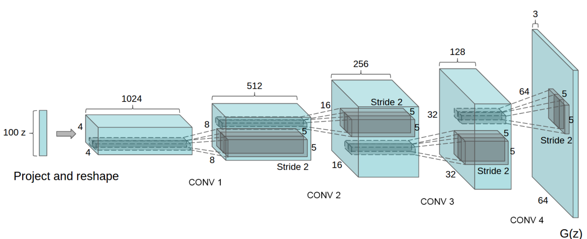The structure of generator (G) in DCGAN is as following:：

figure 3. Generator(G) in DCGAN

## Dataset prepare In this tutorial, we use MNIST to train generator and discriminator, and the dataset can be downloaded to the local automatically through the paddle.dataset module. For detailed introduction of MNIST, please refer to[recognize_digits](https://github.com/PaddlePaddle/book/tree/develop/02.recognize_digits)。 ## Model Training `09.gan/dc_gan.py` shows the whole process of training. ### Import dependency First import necessary dependency. ```python from __future__ import absolute_import from __future__ import division from __future__ import print_function import sys import os import matplotlib import PIL import six import numpy as np import math import time import paddle import paddle.fluid as fluid matplotlib.use('agg') import matplotlib.pyplot as plt import matplotlib.gridspec as gridspec ``` ### Defining auxiliary tool Define plot function to visualize the process of image generated. ```python def plot(gen_data): pad_dim = 1 paded = pad_dim + img_dim gen_data = gen_data.reshape(gen_data.shape[0], img_dim, img_dim) n = int(math.ceil(math.sqrt(gen_data.shape[0]))) gen_data = (np.pad( gen_data, [[0, n * n - gen_data.shape[0]], [pad_dim, 0], [pad_dim, 0]], 'constant').reshape((n, n, paded, paded)).transpose((0, 2, 1, 3)) .reshape((n * paded, n * paded))) fig = plt.figure(figsize=(8, 8)) plt.axis('off') plt.imshow(gen_data, cmap='Greys_r', vmin=-1, vmax=1) return fig ``` ### Define hyper-parameter ```python gf_dim = 64 # the number of basic channels of the generator's feature map. The number of all the channels of feature maps in the generator is a multiple of the number of basic channels df_dim = 64 # the number of basic channels of the discriminator's feature map. The number of all the channels of feature maps in the discriminator is a multiple of the number of basic channels gfc_dim = 1024 * 2 # the dimension of full connection layer of generator dfc_dim = 1024 # the dimension of full connection layer of discriminator img_dim = 28 # size of the input picture NOISE_SIZE = 100 # dimension of input noise LEARNING_RATE = 2e-4 # learning rate of training epoch = 20 # epoch number of training output = "./output_dcgan" # storage path of model and test results use_cudnn = False # use cuDNN or not use_gpu=False # use GPU or not ``` ### Define network architecture - Batch Normalization layer Call `fluid.layers.batch_norm` to implement the bn layer. The activation function uses ReLu by default. ```python def bn(x, name=None, act='relu'): return fluid.layers.batch_norm( x, param_attr=name + '1', bias_attr=name + '2', moving_mean_name=name + '3', moving_variance_name=name + '4', name=name, act=act) ``` - Convolution layer Call `fluid.nets.simple_img_conv_pool` to get the result of convolution and pooling. The kernel size of convolution is 5x5, the pooling window size is 2x2, the window sliding step size is 2, and the activation function type is specified by the specific network structure. ```python def conv(x, num_filters, name=None, act=None): return fluid.nets.simple_img_conv_pool( input=x, filter_size=5, num_filters=num_filters, pool_size=2, pool_stride=2, param_attr=name + 'w', bias_attr=name + 'b', use_cudnn=use_cudnn, act=act) ``` - Fully Connected layer ```python def fc(x, num_filters, name=None, act=None): return fluid.layers.fc(input=x, size=num_filters, act=act, param_attr=name + 'w', bias_attr=name + 'b') ``` - Transpose Convolution Layer In the generator, we need to generate a full-scale image by random sampling values. DCGAN uses the transpose convolution layer for upsampling. In fluid, we call `fluid.layers.conv2d_transpose` to realize transpose convolution. ```python def deconv(x, num_filters, name=None, filter_size=5, stride=2, dilation=1, padding=2, output_size=None, act=None): return fluid.layers.conv2d_transpose( input=x, param_attr=name + 'w', bias_attr=name + 'b', num_filters=num_filters, output_size=output_size, filter_size=filter_size, stride=stride, dilation=dilation, padding=padding, use_cudnn=use_cudnn, act=act) ``` - Discriminator The discriminator uses the real dataset and the fake images generated by the generator to train, and in the training process, try to make the output result of the real data close to 1 and the output result of the fake image close to 0 as far as possible. The discriminator implemented in this tutorial is composed of two convolution_pooling layers and two fully connected layers. The number of neurons in the last fully connected layer is 1, and a binary classification result is output. ```python def D(x): x = fluid.layers.reshape(x=x, shape=[-1, 1, 28, 28]) x = conv(x, df_dim, act='leaky_relu',name='conv1') x = bn(conv(x, df_dim * 2,name='conv2'), act='leaky_relu',name='bn1') x = bn(fc(x, dfc_dim,name='fc1'), act='leaky_relu',name='bn2') x = fc(x, 1, act='sigmoid',name='fc2') return x ``` - Generator The generator consists of two groups of fully connected layers with BN and two groups of transpose convolution layers. The network input is random noise data. The convolution kernel number of the last layer of transposed convolution is 1, indicating that the output is a gray-scale picture. ```python def G(x): x = bn(fc(x, gfc_dim,name='fc3'),name='bn3') x = bn(fc(x, gf_dim * 2 * img_dim // 4 * img_dim // 4,name='fc4'),name='bn4') x = fluid.layers.reshape(x, [-1, gf_dim * 2, img_dim // 4, img_dim // 4]) x = deconv(x, gf_dim * 2, act='relu', output_size=[14, 14],name='deconv1') x = deconv(x, num_filters=1, filter_size=5, padding=2, act='tanh', output_size=[28, 28],name='deconv2') x = fluid.layers.reshape(x, shape=[-1, 28 * 28]) return x ``` ### Loss function Loss function uses `sigmoid_cross_entropy_with_logits` ```python def loss(x, label): return fluid.layers.mean( fluid.layers.sigmoid_cross_entropy_with_logits(x=x, label=label)) ``` ### Create Program ```python d_program = fluid.Program() dg_program = fluid.Program() # Define the program to distinguish the real picture with fluid.program_guard(d_program): # size of the input picture is28*28=784 img = fluid.data(name='img', shape=[None, 784], dtype='float32') # label shape=1 label = fluid.data(name='label', shape=[None, 1], dtype='float32') d_logit = D(img) d_loss = loss(d_logit, label) # Define the program to distinguish the generated pictures with fluid.program_guard(dg_program): noise = fluid.data( name='noise', shape=[None, NOISE_SIZE], dtype='float32') # Noise data as input to generate image g_img = G(x=noise) g_program = dg_program.clone() g_program_test = dg_program.clone(for_test=True) # Judge the probability that the generated image is a real sample dg_logit = D(g_img) # Calculate the loss of the generated image as the real sample noise_shape = fluid.layers.shape(noise) dg_loss = loss( dg_logit, fluid.layers.fill_constant( dtype='float32', shape=[noise_shape[0], 1], value=1.0)) ``` Adam is used as the optimizer to distinguish the loss of the real picture and the loss of the generated picture. ```python opt = fluid.optimizer.Adam(learning_rate=LEARNING_RATE) opt.minimize(loss=d_loss) parameters = [p.name for p in g_program.global_block().all_parameters()] opt.minimize(loss=dg_loss, parameter_list=parameters) ``` ### Dataset Feeders configuration Next, we start the training process. paddle.dataset.mnist.train() is used as training dataset. This function returns a reader. The reader in is a python function, which returns one Python yield generator every time it is called. The shuffle below is a reader decorator. It accepts a reader A and returns another reader B. Reader B reads the buffer_size training data into a buffer every time, then randomly scrambles its order and outputs it one by one. Batch is a special decorator. Its input is a reader and its output is a batched reader. In PaddlePaddle, a reader yields one piece of training data at a time, while a batched reader yields one minibatch at a time. ```python batch_size = 128 # Minibatch size train_reader = fluid.io.batch( fluid.io.shuffle( paddle.dataset.mnist.train(), buf_size=60000), batch_size=batch_size) ``` ### Create actuator ```python if use_gpu: exe = fluid.Executor(fluid.CUDAPlace(0)) else: exe = fluid.Executor(fluid.CPUPlace()) exe.run(fluid.default_startup_program()) ``` ### Start training For each iteration in the training process, the generator and the discriminator set their own iteration times respectively. In order to avoid the discriminator converging to 0 rapidly. In this tutorial, by default, every iteration, the discriminator are trained once and generator twice. ```python t_time = 0 losses = [[], []] # The number of iterations of the discriminator NUM_TRAIN_TIMES_OF_DG = 2 # Noise data of final generated image const_n = np.random.uniform( low=-1.0, high=1.0, size=[batch_size, NOISE_SIZE]).astype('float32') for pass_id in range(epoch): for batch_id, data in enumerate(train_reader()): if len(data) != batch_size: continue # Generating noise data during training noise_data = np.random.uniform( low=-1.0, high=1.0, size=[batch_size, NOISE_SIZE]).astype('float32') # Real image real_image = np.array(list(map(lambda x: x[0], data))).reshape( -1, 784).astype('float32') # Real label real_labels = np.ones( shape=[real_image.shape[0], 1], dtype='float32') # Fake label fake_labels = np.zeros( shape=[real_image.shape[0], 1], dtype='float32') total_label = np.concatenate([real_labels, fake_labels]) s_time = time.time() # Fake image generated_image = exe.run(g_program, feed={'noise': noise_data}, fetch_list=[g_img])[0] total_images = np.concatenate([real_image, generated_image]) # D loss of judging fake pictures as fake d_loss_1 = exe.run(d_program, feed={ 'img': generated_image, 'label': fake_labels, }, fetch_list=[d_loss])[0][0] # D loss of judging true pictures as true d_loss_2 = exe.run(d_program, feed={ 'img': real_image, 'label': real_labels, }, fetch_list=[d_loss])[0][0] d_loss_n = d_loss_1 + d_loss_2 losses[0].append(d_loss_n) # Training generator for _ in six.moves.xrange(NUM_TRAIN_TIMES_OF_DG): noise_data = np.random.uniform( low=-1.0, high=1.0, size=[batch_size, NOISE_SIZE]).astype('float32') dg_loss_n = exe.run(dg_program, feed={'noise': noise_data}, fetch_list=[dg_loss])[0][0] losses[1].append(dg_loss_n) t_time += (time.time() - s_time) if batch_id % 10 == 0 : if not os.path.exists(output): os.makedirs(output) # Results of each round generated_images = exe.run(g_program_test, feed={'noise': const_n}, fetch_list=[g_img])[0] # Connect real pictures to generated pictures total_images = np.concatenate([real_image, generated_images]) fig = plot(total_images) msg = "Epoch ID={0} Batch ID={1} D-Loss={2} DG-Loss={3}\n ".format( pass_id, batch_id, d_loss_n, dg_loss_n) print(msg) plt.title(msg) plt.savefig( '{}/{:04d}_{:04d}.png'.format(output, pass_id, batch_id), bbox_inches='tight') plt.close(fig) ``` Print the results of a specific round: ```python def display_image(epoch_no,batch_id): return PIL.Image.open('output_dcgan/{:04d}_{:04d}.png'.format(epoch_no,batch_id)) # Observe the generated images of the 10th epoch and 460 batches: display_image(10,460) ``` ## Summary DCGAN use a random noise vector as the input, the input is amplified into two-dimensional data through a similar but opposite structure to CNN. By using the generative model of this structure and the discriminative model of CNN structure, DCGAN can achieve considerable results in image generative. In this case, we use DCGAN to generate handwritten digital images. You can try to change dataset to generate images that meet your personal needs, or try to modify the network structure to observe different generative effects. ## Reference [1] Goodfellow, Ian J.; Pouget-Abadie, Jean; Mirza, Mehdi; Xu, Bing; Warde-Farley, David; Ozair, Sherjil; Courville, Aaron; Bengio, Yoshua. Generative Adversarial Networks. 2014. arXiv:1406.2661 [stat.ML]. [2] Andrej Karpathy, Pieter Abbeel, Greg Brockman, Peter Chen, Vicki Cheung, Rocky Duan, Ian Goodfellow, Durk Kingma, Jonathan Ho, Rein Houthooft, Tim Salimans, John Schulman, Ilya Sutskever, And Wojciech Zaremba, Generative Models, OpenAI, [April 7, 2016] [3] alimans, Tim; Goodfellow, Ian; Zaremba, Wojciech; Cheung, Vicki; Radford, Alec; Chen, Xi. Improved Techniques for Training GANs. 2016. arXiv:1606.03498 [cs.LG]. [4] Radford A, Metz L, Chintala S. Unsupervised Representation Learning with Deep Convolutional Generative Adversarial Networks[J]. Computer Science, 2015.