Fixed-point quantization uses lower bits, for example, 2-bit, 3-bit or 8-bit fixed point to represent weights and activations, which usually are in singe-precision float-point with 32 bits. The fixed-point representation has advantages in reducing memory bandwidth, lowering power consumption and computational resources as well as the model storage requirements.  It is especially important for the inference in embedded-device deployment.

According to some experiments, the apporach to quantize the model trained in float point directly works effectively on the large models, like the VGG model having many parameters. But the accuracy drops a lot for the small model. In order to improve the tradeoff between accuracy and latency, many quantized training apporaches are proposed.

This document is to design a quantized training framework on Fluid. The first part will introduce how to quantize, The second part will describe the quantized training framework. The last part will illustrate how to calculate the quantization scale.


### How to quantize

There are many ways to quantize the float value to fixed-point value. For example:

$$ r = min(max(x, a), b)$$
$$ s = \frac{b - a}{n - 1} $$
$$ q = \left \lfloor \frac{r - a}{s} \right \rceil $$

where, $x$ is the float value to be quantized, $[a, b]$ is the quantization range, $a$ is the minimum value and $b$ is the maximal value. $\left \lfloor \right \rceil$  denotes rounding to the nearest integer. If the quantization level is $k$, $n$ is $2^k$, for example, $k$ is 8 and $n$ is 256. $q$ is the quantized integer. 


The quantization we applied is parameterized by the number of quantization levels and maximum absolute value:

$$ M  = max(abs(x))  $$
$$ q = \left \lfloor \frac{x}{M} * (n - 1) \right \rceil $$

where, $x$ is the float value to be quantized, $M$ is maximum absolute value. $\left \lfloor \right \rceil$ denotes rounding to the nearest integer.  For 8 bit quantization, $n=2^{8}=256$. $q$ is the quantized integer. 


Wether the *min-max* quantization or *max-abs* quantization, they also can be represent:

$q = scale * r + b$

We call *min-max*, *max-abs* as the quantization arguments, also call them quantization scale or quantization range.


How to calculate the quantization scale (or maximum absolute value) for inference will be described in the last part.


### Training Framework

#### Forward pass

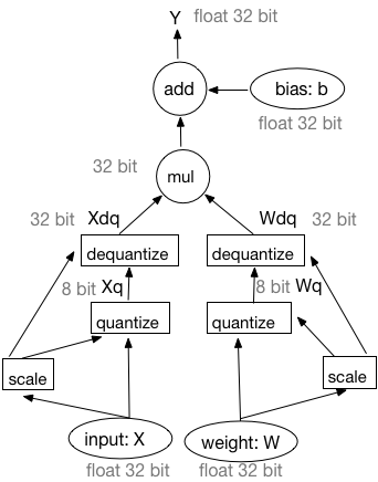
The forward pass is simulated quantization, see Figure 1.

The training framework is as following figure. 

<p align="center"> 
<img src="quantization_forward.png" width="300" height="340"><br/>
Figure 1. Forward in training with simulated quantization.
</p>

- Firstly, both input and weight will be quantized to 8-bit integers. 
- Second, do the multiplication (or convolution) operation with integers.
- Third, dequantize the multiplication (or convolution) results to 32-bit float point.
- Finally, do bias-addition in float type of 32 bit. Here, the bias is not quantized.

For general matrix multiplication (GEMM), quantize for $X$ and $W$:

$$ X_q = \left \lfloor \frac{X}{X_m} * (n - 1) \right \rceil  $$
$$ W_q = \left \lfloor \frac{W}{W_m} * (n - 1) \right \rceil $$

Do GEMM:

$$ Y = X_q * W_q $$


Dequantize $Y$:

$$
\begin{align}
Y_{dq} &=\frac{Y}{(n - 1) * (n - 1)} * X_m * W_m \\\
       &=\frac{X_q * W_q}{(n - 1) * (n - 1)} * X_m * W_m \\\
       &=(\frac{X_q}{n - 1} * X_m) * (\frac{W_q}{n - 1} * W_m) 
\end{align}
$$

From these formulas, dequantization also can be moved before GEMM, do dequantization for $Xq$ and $Wq$ at first, then do GEMM. The forward workflow in training is equivalent to following framework.

<p align="center"> 
<img src="quantization_equivalent_forward.png"  width="300" height="330"><br/>
Figure 2. Equivalent forward in training with simulated quantization.
</p>

We use this equivalent workflow in the training. In our desigin, there is a quantization transpiler to insert the quantization operator and the de-quantization operator in the Fluid `ProgramDesc`. Since the outputs of quantization and de-quantization operator are still in floating point, they are called faked quantization and de-quantization operator. And the training framework is called simulated quantization.

#### Backward pass

See Figure 3. The gradients are calculated by dequantized weights and activations. All inputs and outputs are float point with 32-bit. And in the weight updating process, the gradients will be added to the original weight, not the quantized or dequantized weights.

<p align="center"> 
<img src="quantization_backward_and_optimization.png"><br/>
Figure 3. Backward and weight updating in training with simulated quantization.
</p>

So the quantization transipler will change some inputs of the corresponding backward operators. 

### How to calculate quantization scale

There are two strategies to calculate quantization scale, we call them dynamic and static strategy. The dynamic strategy calculates the quantization scale value each iteration. The static strategy keeps the quantization scale for different inputs.

For weights, we apply the dynamic strategy in the training, that is to say, the quantization scale will be recalculated during each iteration until the traning is finished.

For activations, the quantization scales are estimated during training, then used in inference. There are several different ways to estimate them:


1. Calculate the mean of maximum absolute during a window.
2. Calculate the max of maximum absolute during a window.
3. Calculate the running mean of maximum absolute during a window, as follows:

    $$ Vt = (1 - k) * V +  k * V_{t-1}  $$
    
    where, $V$ is the maximum absolute value of current batch, $Vt$ is the running mean value. $k$ is a factor, such as 0.9.